14.4 Stem-and-Leaf Diagrams and Histograms
SL 4.2
- how to draw and read an ordered stem-and-leaf diagram
- how to draw and read frequency histograms for discrete data and for grouped continuous data (equal class widths)
- how to draw a frequency polygon
- the differences between a histogram and a bar chart
Stem-and-leaf diagrams
A stem-and-leaf diagram shows every value in a data set, but in a compact, organised way. Each value is split into a stem (usually the tens digit) and a leaf (the units digit).
For example, \(47\) is written with stem \(4\) and leaf \(7\):
4 | 7Many values can share one stem. Each leaf is written in the row of its stem. For the data \(52, 47, 58, 61, 43, 52, 55\):
4 | 3 7
5 | 2 2 5 8
6 | 1          Key: 5 | 2 means 52
Rules for a stem-and-leaf diagram
- Write the leaves in ascending order (an ordered diagram), so the median is easy to find.
- If a value appears more than once, write a leaf for each time it appears (52 appears twice above).
- Always include a key.
A stem-and-leaf diagram keeps the original values, and its shape is like a histogram turned on its side.
Example 1 The times (in minutes) taken by 16 students to travel to school are:
\[ 23,\ 8,\ 35,\ 17,\ 42,\ 26,\ 31,\ 14,\ 29,\ 9,\ 38,\ 21,\ 27,\ 15,\ 33,\ 26 \]
(a) Draw an ordered stem-and-leaf diagram.
(b) Find the median.
(c) Find the range.
(a) Use the tens digit as the stem (8 and 9 have stem 0):
0 | 8 9
1 | 4 5 7
2 | 1 3 6 6 7 9
3 | 1 3 5 8
4 | 2          Key: 2 | 1 means 21 minutes
(b) \(n = 16\), so the median is halfway between the 8th and 9th values. Counting along the rows: \(8, 9, 14, 15, 17, 21, 23, \mathbf{26}, \mathbf{26}, \ldots\) The median is \(26\) minutes.
(c) Range \(= 42 - 8 = 34\) minutes.
Histograms
A frequency histogram shows how the data are distributed. The horizontal axis is a number line (a continuous scale) and the height of each column is the frequency.
For discrete data, each column is centred on one value. Figure 1 shows the number of pets owned by 20 families.
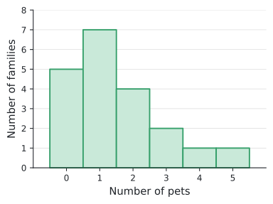
From the histogram: the tallest column is at \(1\), so the mode is 1 pet. Five families have no pets, and only \(1 + 1 = 2\) families have more than 3 pets.
For grouped continuous data, each column covers one class, from its lower boundary to its upper boundary. At SL, histograms have equal class widths, so the height of each column is the frequency.
Frequency polygons
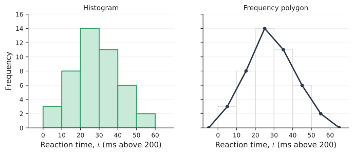
A frequency polygon shows the same information as a histogram. Plot each frequency above the mid-interval value of its class (the middle of the top of each column), and join the points with straight lines. The polygon is usually closed by joining it to the horizontal axis at the mid-points of the empty classes at each end.
Example 2 The histogram shows the distribution of some values of \(p\).
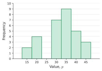
(a) Copy and complete the grouped frequency table.
| Class | Mid-interval value | Frequency |
|---|---|---|
| \(12.5 \le p < 17.5\) | 15 | |
| \(17.5 \le p < 22.5\) | 20 | |
| \(22.5 \le p < 27.5\) | 25 | |
| \(27.5 \le p < 32.5\) | 30 | |
| \(32.5 \le p < 37.5\) | 35 | |
| \(37.5 \le p < 42.5\) | 40 | |
| \(42.5 \le p < 47.5\) | 45 |
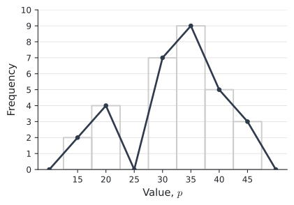
(b) Draw a frequency polygon for the data.
(c) How many values are in the class \(27.5 \le p < 32.5\)?
(d) How many values are less than \(32.5\)?
(e) Write down the modal class.
(a) Read the height of each column: \(2, 4, 0, 7, 9, 5, 3\) (total \(30\)).
(b) Plot the points \((15, 2), (20, 4), (25, 0), (30, 7), (35, 9), (40, 5), (45, 3)\) and join them, closing the polygon at \((10, 0)\) and \((50, 0)\).
(c) \(7\).
(d) \(2 + 4 + 0 + 7 = 13\).
(e) \(32.5 \le p < 37.5\) (the tallest column).
A histogram is not a bar chart
A histogram looks like a bar chart, but they are used for different things.
| Histogram | Bar chart |
|---|---|
| Shows the distribution of numerical data | Compares the sizes of categories |
| Numerical (quantitative) data | Categorical (qualitative) data, such as favourite colour |
| Both axes have a numerical scale | Only the vertical axis has a numerical scale |
| No gaps between columns | Gaps between bars |
| Columns cannot be re-ordered: each covers part of a number line | Bars can be put in any order |
Key features of a histogram Not in the formula booklet
- The horizontal axis is a continuous number scale divided into class intervals.
- The vertical axis shows frequency.
- There are no gaps between columns. A class with frequency \(0\) is shown as an empty space of the same width — that is not a gap between columns.
- With equal class widths, the height of each column is proportional to its frequency.
When classes have different widths, it is the area of each column (not its height) that should be proportional to the frequency. The height is then the frequency density:
\[ \text{frequency density} = \frac{\text{frequency}}{\text{class width}} . \]
For example, a class \(20 \le t < 40\) with frequency 30 has height \(\frac{30}{20} = 1.5\), while a class \(40 \le t < 45\) with frequency 15 has height \(\frac{15}{5} = 3\).
The IB syllabus says frequency density histograms are not required; exam histograms have equal class widths.
Common errors
| ✗ Wrong | ✓ Right | Why |
|---|---|---|
| Leaves not in order | Ordered leaves | Ordered leaves make the median easy to find. |
| No key on a stem-and-leaf diagram | Always give a key | “\(2 \mid 1\)” could mean 21, 2.1 or 210. |
| Gaps between histogram columns | No gaps | The horizontal axis is a continuous scale. |
| Polygon points at class boundaries | Points at mid-interval values | Each point stands for a whole class. |
| Bar chart for heights of students | Histogram | Height is numerical, continuous data. |
Exercises
1 The marks of 18 students are: \(52, 38, 47, 61, 45, 53, 39, 58, 44, 50, 63, 47, 55, 41, 49, 57, 36, 52\).
(a) Draw an ordered stem-and-leaf diagram.
(b) Find the median and the range.
(a)
3 | 6 8 9
4 | 1 4 5 7 7 9
5 | 0 2 2 3 5 7 8
6 | 1 3          Key: 4 | 1 means 41
(b) Median: halfway between the 9th and 10th values, \(49\) and \(50\): median \(= 49.5\). Range \(= 63 - 36 = 27\).
2 Explain why the columns of a histogram cannot be put in a different order, but the bars of a bar chart can.
Each column of a histogram covers a fixed interval of a number line, so its position is fixed by the values. The bars of a bar chart are separate categories with no natural order, so they can be arranged in any order.
3 A histogram of the ages of 40 people has equal class widths of 10 years. The heights of the columns for \(10 \le a < 20\), \(20 \le a < 30\), \(30 \le a < 40\), \(40 \le a < 50\) and \(50 \le a < 60\) are \(4, 0, 11, x, 7\).
(a) Find \(x\). \(\qquad\) (b) What percentage of the people are under 40?
(a) \(4 + 0 + 11 + x + 7 = 40\), so \(x = 18\).
(b) \(\dfrac{4 + 0 + 11}{40} \times 100\% = 37.5\%\).
4 A frequency polygon has its points at \((15, 4), (25, 9), (35, 12), (45, 5)\). The classes have width 10.
(a) Write down the classes and frequencies.
(b) Find the total frequency.
(c) Estimate the mean.
(a) \(10 \le x < 20\): 4; \(\;20 \le x < 30\): 9; \(\;30 \le x < 40\): 12; \(\;40 \le x < 50\): 5.
(b) \(30\).
(c) \(\dfrac{4(15) + 9(25) + 12(35) + 5(45)}{30} = \dfrac{930}{30} = 31\).