12.1 Translations, Stretches and Reflections
SL 2.11
- what a transformation of a graph is
- how the graphs of \(y = f(x) + b\) and \(y = f(x - a)\) are related to the graph of \(y = f(x)\) (translations)
- how to describe a translation with a translation vector \(\begin{pmatrix} a \\ b \end{pmatrix}\)
- how the graphs of \(y = p\,f(x)\) and \(y = f(qx)\) are related to the graph of \(y = f(x)\) (stretches)
- how the graphs of \(y = -f(x)\) and \(y = f(-x)\) are related to the graph of \(y = f(x)\) (reflections)
- which points do not move (invariant points)
- how to find the images of points, turning points, intercepts and asymptotes after a transformation
Transformations
If we know the graph of \(y = f(x)\), we can draw many other graphs from it without plotting new points. We move, stretch or reflect the graph. Each of these changes is called a transformation.
In this unit, the original graph is drawn as a grey dashed curve, and the new graph (the image) is drawn in colour.
There are three basic kinds of transformation:
- a translation slides the graph. It does not change its shape or size.
- a stretch makes the graph taller or shorter, or wider or narrower.
- a reflection flips the graph over one of the axes.
Translations
Vertical translation
Start with \(f(x) = x^2\). The graph of \(y = x^2 + 3\) has every \(y\)-value 3 bigger than the graph of \(y = x^2\). So the whole curve moves up 3 units. In the same way, \(y = x^2 - 2\) is the curve moved down 2 units.
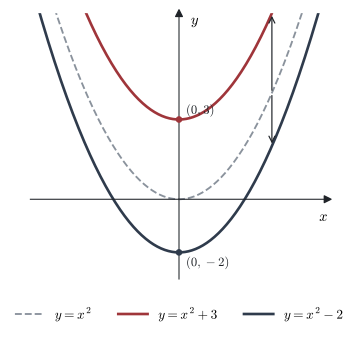
Vertical translation Not in the formula booklet
The graph of \(y = f(x) + b\) is the graph of \(y = f(x)\) translated \(b\) units parallel to the \(y\)-axis.
- \(b > 0\): the graph moves up \(b\) units.
- \(b < 0\): the graph moves down \(|b|\) units.
Each point moves like this: \(\quad (x,\, y) \;\longmapsto\; (x,\, y + b)\).
- \(b\): the number added outside \(f\) (the movement in the \(y\)-direction)
Horizontal translation
Now compare \(y = x^2\) with \(y = (x + 3)^2\) and \(y = (x - 2)^2\).
- \(y = (x + 3)^2\) is zero when \(x = -3\). Its vertex is at \((-3, 0)\): the curve has moved left 3 units.
- \(y = (x - 2)^2\) is zero when \(x = 2\). Its vertex is at \((2, 0)\): the curve has moved right 2 units.
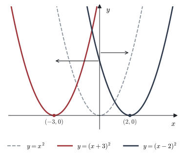
Why does “\(-2\)” move the graph to the right? On the new graph, \(y = f(x - 2)\). To get the same \(y\)-value as \(f\) gives at \(x = 0\), we now need \(x - 2 = 0\), so \(x = 2\). Every \(y\)-value now appears 2 units later.
Horizontal translation Not in the formula booklet
The graph of \(y = f(x - a)\) is the graph of \(y = f(x)\) translated \(a\) units parallel to the \(x\)-axis.
- \(a > 0\), for example \(y = f(x - 2)\): the graph moves right \(a\) units.
- \(a < 0\), for example \(y = f(x + 3)\): the graph moves left \(|a|\) units.
Each point moves like this: \(\quad (x,\, y) \;\longmapsto\; (x + a,\, y)\).
- \(a\): the number subtracted from \(x\) inside \(f\) (the movement in the \(x\)-direction)
Important points about translations
- The shape of the curve does not change. Only its position changes.
- Asymptotes move too. A horizontal asymptote \(y = k\) moves with a vertical translation. A vertical asymptote \(x = h\) moves with a horizontal translation.
Example 1 The graph of \(y = f(x)\) passes through the origin \(O\), the points \(A(2, 2)\) and \(B(-2, -2)\). It has a maximum point \(P(-1, 2)\) and a minimum point \(Q(1, -2)\).
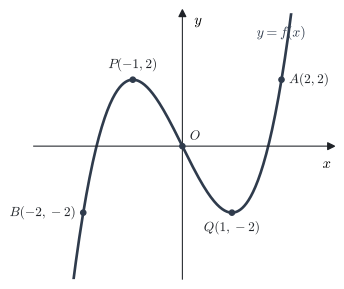
Sketch, on separate diagrams, the graphs of
(a) \(y = f(x) + 3\)
(b) \(y = f(x) - 2\)
(c) \(y = f(x - 1)\)
(d) \(y = f(x + 2)\)
Label the images of \(O\), \(A\), \(B\), \(P\) and \(Q\).
Use the point rules: (a) and (b) change only the \(y\)-coordinate; (c) and (d) change only the \(x\)-coordinate.
| Point | (a) \((x, y + 3)\) | (b) \((x, y - 2)\) | (c) \((x + 1, y)\) | (d) \((x - 2, y)\) |
|---|---|---|---|---|
| \(O(0, 0)\) | \((0, 3)\) | \((0, -2)\) | \((1, 0)\) | \((-2, 0)\) |
| \(A(2, 2)\) | \((2, 5)\) | \((2, 0)\) | \((3, 2)\) | \((0, 2)\) |
| \(B(-2, -2)\) | \((-2, 1)\) | \((-2, -4)\) | \((-1, -2)\) | \((-4, -2)\) |
| \(P(-1, 2)\) max | \((-1, 5)\) | \((-1, 0)\) | \((0, 2)\) | \((-3, 2)\) |
| \(Q(1, -2)\) min | \((1, 1)\) | \((1, -4)\) | \((2, -2)\) | \((-1, -2)\) |
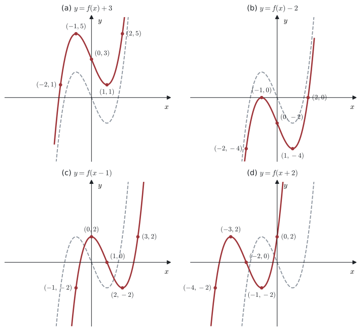
In (b) the maximum point moves onto the \(x\)-axis, so the new graph touches the \(x\)-axis at \((-1, 0)\). In (c) the maximum point moves onto the \(y\)-axis, so \((0, 2)\) is the \(y\)-intercept.
Example 2 The curve \(C\) has equation \(y = f(x)\). It has asymptotes \(x = 0\) and \(y = 0\), a minimum point \(A(-4, -1)\) and an \(x\)-intercept \(B(-2, 0)\). The curve \(C_1\) has the same shape.
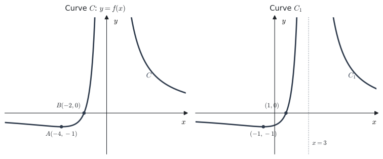
(a) Write down the equation of \(C_1\) in terms of \(f\).
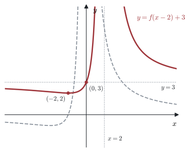
(b) Hence sketch the graph of \(y = f(x - 2) + 3\). Show the asymptotes, the axis intercepts and the images of \(A\) and \(B\).
(a) The vertical asymptote has moved from \(x = 0\) to \(x = 3\). The minimum point has moved from \((-4, -1)\) to \((-1, -1)\), and the intercept from \((-2, 0)\) to \((1, 0)\). Every point has moved 3 units right and the \(y\)-values are the same. So \(C_1\) is \(y = f(x - 3)\).
(b) \(y = f(x - 2) + 3\): move 2 right and 3 up, \((x, y) \longmapsto (x + 2, y + 3)\).
- Asymptotes: \(x = 0 \to x = 2\) and \(y = 0 \to y = 3\).
- \(A(-4, -1) \to (-2, 2)\), a minimum point.
- \(B(-2, 0) \to (0, 3)\). This point is on the \(y\)-axis, so the \(y\)-intercept is \((0, 3)\).
- The lowest point of the new curve is at \(y = 2 > 0\), and the right-hand part is above \(y = 3\). So the new graph has no \(x\)-intercepts.
Translation vectors
A translation is often written as a column vector. The top number is the movement in the \(x\)-direction, and the bottom number is the movement in the \(y\)-direction.
Translation by a vector Not in the formula booklet
The graph of \(y = f(x - a) + b\) is the graph of \(y = f(x)\) translated by the vector \(\begin{pmatrix} a \\ b \end{pmatrix}\).
Each point moves like this: \(\quad (x,\, y) \;\longmapsto\; (x + a,\, y + b)\).
- \(a\): the movement parallel to the \(x\)-axis (positive = right)
- \(b\): the movement parallel to the \(y\)-axis (positive = up)
To find the new equation, replace \(x\) by \(x - a\), then add \(b\).
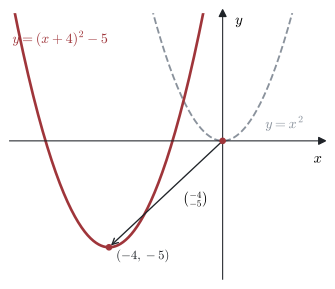
Example 3 (a) Describe the transformation that maps the graph of \(y = x^2\) onto the graph of \(y = (x + 4)^2 - 5\).
(b) The graph of \(y = x^3 - 2x\) is translated by the vector \(\begin{pmatrix} -1 \\ 3 \end{pmatrix}\). Find the equation of the new graph in the form \(y = x^3 + px^2 + qx + r\).
(a) \((x + 4)^2 - 5 = f(x - (-4)) + (-5)\) with \(f(x) = x^2\). This is a translation by the vector \(\begin{pmatrix} -4 \\ -5 \end{pmatrix}\): 4 units left and 5 units down. The vertex moves from \((0, 0)\) to \((-4, -5)\).
(b) Replace \(x\) by \(x + 1\), then add \(3\):
\[ \begin{aligned} y &= (x + 1)^3 - 2(x + 1) + 3 \\ &= x^3 + 3x^2 + 3x + 1 - 2x - 2 + 3 \\ &= x^3 + 3x^2 + x + 2 . \end{aligned} \]
- Open a Graphs page.
- Enter \(f_1(x) = x^3 - 2x\).
- Enter \(f_2(x) = f_1(x + 1) + 3\). The calculator accepts \(f_1\) inside \(f_2\), so you do not need to expand.
- Enter \(f_3(x) = x^3 + 3x^2 + x + 2\) (your expanded answer).
- If your expansion is right, the graphs of \(f_2\) and \(f_3\) lie exactly on top of each other.
- To compare values, press ctrl + T to show a table: the columns for \(f_2\) and \(f_3\) must be the same.
The same idea checks any stretch or reflection, for example \(f_2(x) = 2 f_1(x)\) or \(f_2(x) = f_1(-x)\).
Stretches
A stretch is described by a direction (parallel to the \(x\)-axis or parallel to the \(y\)-axis) and a scale factor.
- A scale factor greater than 1 pulls the graph away from an axis.
- A scale factor between 0 and 1 pushes the graph towards an axis (it squashes the graph). We still call this a stretch.
Vertical stretch
Let \(f(x) = x^3 - 4x = x(x - 2)(x + 2)\). For \(y = 2f(x)\), every \(y\)-value is doubled. For \(y = \frac{1}{3}f(x)\), every \(y\)-value is one third of the old value. The \(x\)-values do not change.
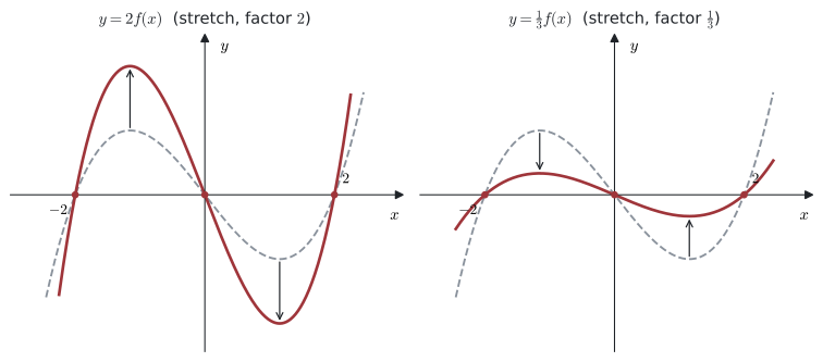
Look at the points on the \(x\)-axis: \((-2, 0)\), \((0, 0)\) and \((2, 0)\). Since \(2 \times 0 = 0\), they do not move. They are invariant points.
Vertical stretch Not in the formula booklet
The graph of \(y = p\,f(x)\) (with \(p > 0\)) is the graph of \(y = f(x)\) stretched parallel to the \(y\)-axis with scale factor \(p\).
Each point moves like this: \(\quad (x,\, y) \;\longmapsto\; (x,\, p\,y)\).
Points on the \(x\)-axis are invariant. A horizontal asymptote \(y = k\) becomes \(y = pk\); vertical asymptotes do not move.
- \(p\): the number multiplying \(f(x)\) outside \(f\) (the scale factor)
- \(k\): the height of a horizontal asymptote of \(y = f(x)\)
You may also see the equation written with \(y\) replaced. If \(a\,y = f(x)\), then \(y = \frac{1}{a}f(x)\). So replacing \(y\) by \(ay\) gives a stretch parallel to the \(y\)-axis with scale factor \(\frac{1}{a}\).
Horizontal stretch
Let \(f(x) = (x - 1)(x - 3) = x^2 - 4x + 3\). Its roots are \(1\) and \(3\), its vertex is \((2, -1)\) and its \(y\)-intercept is \((0, 3)\).
- \(y = f(2x) = (2x - 1)(2x - 3)\) has roots \(\frac{1}{2}\) and \(\frac{3}{2}\). The graph is squashed towards the \(y\)-axis: every \(x\)-value is halved.
- \(y = f\left(\frac{1}{2}x\right)\) has roots \(2\) and \(6\). The graph is pulled away from the \(y\)-axis: every \(x\)-value is doubled.
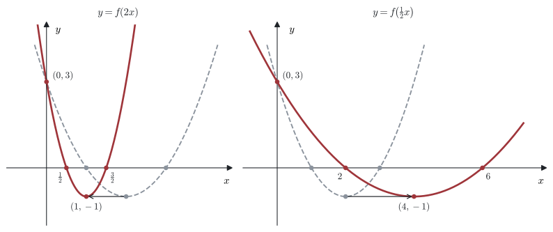
Why is the factor upside down? On \(y = f(2x)\), we get the old value \(f(3)\) when \(2x = 3\), that is when \(x = \frac{3}{2}\). So each \(y\)-value appears at half the old \(x\)-value.
The point \((0, 3)\) on the \(y\)-axis does not move, because \(2 \times 0 = 0\).
Horizontal stretch Not in the formula booklet
The graph of \(y = f(qx)\) (with \(q > 0\)) is the graph of \(y = f(x)\) stretched parallel to the \(x\)-axis with scale factor \(\dfrac{1}{q}\).
Each point moves like this: \(\quad (x,\, y) \;\longmapsto\; \left(\dfrac{x}{q},\, y\right)\).
Points on the \(y\)-axis are invariant. A vertical asymptote \(x = h\) becomes \(x = \frac{h}{q}\); horizontal asymptotes do not move.
- \(q\): the number multiplying \(x\) inside \(f\) (the scale factor is \(\frac{1}{q}\))
- \(h\): the position of a vertical asymptote of \(y = f(x)\)
Important points about stretches
- A stretch changes the size of the curve in one direction, but the general shape (number of turning points, asymptotes) stays.
- \(y = p\,f(x)\): the change is outside \(f\), so it acts on \(y\), and it does what it says (multiply \(y\) by \(p\)).
- \(y = f(qx)\): the change is inside \(f\), so it acts on \(x\), and it does the opposite (divide \(x\) by \(q\)).
Example 4 The graph of \(y = f(x)\) has asymptotes \(x = 2\) and \(y = 1\). It crosses the \(y\)-axis at \(\left(0, \frac{5}{2}\right)\) and the \(x\)-axis at \((5, 0)\).
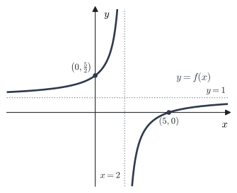
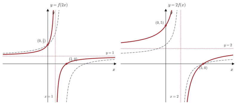
Sketch, on separate diagrams, the graphs of \(\;y = f(2x)\;\) and \(\;y = 2f(x)\). Show the asymptotes and the axis intercepts.
\(y = f(2x)\): stretch parallel to the \(x\)-axis, scale factor \(\frac{1}{2}\): \((x, y) \longmapsto \left(\frac{x}{2}, y\right)\).
- Vertical asymptote \(x = 2 \to x = 1\). The horizontal asymptote \(y = 1\) does not change.
- \(\left(0, \frac{5}{2}\right)\) is on the \(y\)-axis, so it is invariant. \((5, 0) \to \left(\frac{5}{2}, 0\right)\).
\(y = 2f(x)\): stretch parallel to the \(y\)-axis, scale factor \(2\): \((x, y) \longmapsto (x, 2y)\).
- Horizontal asymptote \(y = 1 \to y = 2\). The vertical asymptote \(x = 2\) does not change.
- \(\left(0, \frac{5}{2}\right) \to (0, 5)\). \(\;(5, 0)\) is on the \(x\)-axis, so it is invariant.
Example 5 The curve \(C_1\) is the circle \(x^2 + y^2 = 4\). The curve \(C_2\) is an ellipse that meets the axes at \((\pm 2, 0)\) and \((0, \pm 3)\).
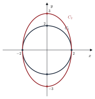
(a) Describe fully the single transformation that maps \(C_1\) onto \(C_2\).
(b) Find the equation of \(C_2\).
(a) The points \((\pm 2, 0)\) on the \(x\)-axis do not move. The point \((0, 2)\) moves to \((0, 3)\). So \(C_2\) is a stretch parallel to the \(y\)-axis with scale factor \(\dfrac{3}{2}\).
(b) Under this stretch, \((x, y) \longmapsto \left(x, \frac{3}{2}y\right)\). A point \((X, Y)\) on \(C_2\) comes from the point \(\left(X, \frac{2}{3}Y\right)\) on \(C_1\). So we replace \(y\) by \(\frac{2}{3}y\) in the equation of \(C_1\):
\[ \begin{gathered} x^2 + \left(\frac{2y}{3}\right)^2 = 4 \\ x^2 + \frac{4y^2}{9} = 4 \\ \frac{x^2}{4} + \frac{y^2}{9} = 1 \end{gathered} \]
(This is the same rule as before: a stretch with scale factor \(p\) parallel to the \(y\)-axis replaces \(y\) by \(\frac{y}{p}\).)
Reflections
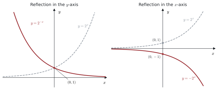
Consider the curve \(C\) with equation \(y = f(x) = 2^x\).
- Replace \(x\) by \(-x\): \(\;y = 2^{-x}\). The value that \(C\) has at \(x = 1\), the new curve has at \(x = -1\). The left and right sides swap. This is a reflection in the \(y\)-axis.
- Replace \(y\) by \(-y\): \(\;-y = 2^x\), that is \(y = -2^x\). Every \(y\)-value changes sign. The top and bottom swap. This is a reflection in the \(x\)-axis.
Reflections Not in the formula booklet
\(y = -f(x)\) is the graph of \(y = f(x)\) reflected in the \(x\)-axis: \(\quad (x,\, y) \;\longmapsto\; (x,\, -y)\). Points on the \(x\)-axis are invariant.
\(y = f(-x)\) is the graph of \(y = f(x)\) reflected in the \(y\)-axis: \(\quad (x,\, y) \;\longmapsto\; (-x,\, y)\). Points on the \(y\)-axis are invariant.
Notice what happens to turning points.
- Under \(y = -f(x)\), a maximum point becomes a minimum point, and a minimum becomes a maximum.
- Under \(y = f(-x)\), a maximum stays a maximum and a minimum stays a minimum. They only change sides.
If we do both reflections, \(y = -f(-x)\), then \((x, y) \longmapsto (-x, -y)\). This is the same as a rotation of \(180^\circ\) about the origin.
Example 6 The graph of \(y = f(x)\) crosses the \(x\)-axis at \((-2, 0)\), has a maximum point \((-1, 4)\), crosses the \(y\)-axis at \((0, 2)\) and has a minimum point \((1, 0)\).
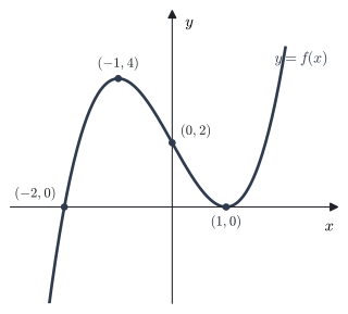
Sketch, on separate diagrams, the graphs of
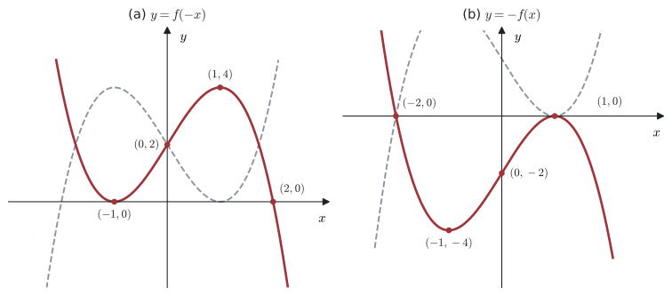
(a) \(y = f(-x)\) \(\qquad\) (b) \(y = -f(x)\)
(a) \((x, y) \longmapsto (-x, y)\): \((-2, 0) \to (2, 0)\), maximum \((-1, 4) \to (1, 4)\), \((0, 2)\) is invariant, minimum \((1, 0) \to (-1, 0)\).
(b) \((x, y) \longmapsto (x, -y)\): \((-2, 0)\) is invariant, the maximum \((-1, 4)\) becomes a minimum \((-1, -4)\), \((0, 2) \to (0, -2)\), and the minimum \((1, 0)\) becomes a maximum \((1, 0)\) (it is on the \(x\)-axis, so it does not move).
Example 7 The graph of \(y = f(x)\) has asymptotes \(x = 1\) and \(y = 2\). It passes through \(A(0, 6)\), \(B(3, 0)\) and \(C(5, 1)\).
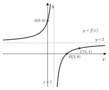
Sketch the graph of \(y = -f(-x)\). State the coordinates of the images of \(A\), \(B\) and \(C\), and the equations of the asymptotes.
Both coordinates change sign: \((x, y) \longmapsto (-x, -y)\).
- \(A(0, 6) \to (0, -6)\), \(\quad B(3, 0) \to (-3, 0)\), \(\quad C(5, 1) \to (-5, -1)\).
- Asymptotes: \(x = 1 \to x = -1\) and \(y = 2 \to y = -2\).
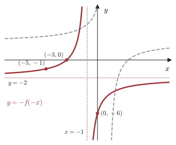
You can do it in two steps: first reflect in the \(y\)-axis (\(y = f(-x)\)), then reflect the result in the \(x\)-axis.
Summary of the basic transformations
| Equation | Transformation of \(y = f(x)\) | Image of a point \((x, y)\) |
|---|---|---|
| \(y = f(x) + b\) | Translation \(b\) units parallel to the \(y\)-axis | \((x,\; y + b)\) |
| \(y = f(x - a)\) | Translation \(a\) units parallel to the \(x\)-axis | \((x + a,\; y)\) |
| \(y = f(x - a) + b\) | Translation by the vector \(\begin{pmatrix} a \\ b \end{pmatrix}\) | \((x + a,\; y + b)\) |
| \(y = p\,f(x)\) | Stretch parallel to the \(y\)-axis, scale factor \(p\) | \((x,\; py)\) |
| \(y = f(qx)\) | Stretch parallel to the \(x\)-axis, scale factor \(\frac{1}{q}\) | \(\left(\frac{x}{q},\; y\right)\) |
| \(y = -f(x)\) | Reflection in the \(x\)-axis | \((x,\; -y)\) |
| \(y = f(-x)\) | Reflection in the \(y\)-axis | \((-x,\; y)\) |
A useful pattern: a change outside \(f\) acts on \(y\) and does what it says. A change inside \(f\) acts on \(x\) and does the opposite (\(-a\) moves right, \(\times q\) divides by \(q\)).
To combine two or more of these transformations, see Section 12.2.
Common errors
| ✗ Wrong | ✓ Right | Why |
|---|---|---|
| \(y = f(x - 3)\) moves the graph left 3 | It moves the graph right 3 | The new graph reaches each \(y\)-value when \(x - 3\) equals the old \(x\), so 3 units later. |
| \(y = f(x) + 2\) and \(y = f(x + 2)\) are the same | \(+2\) outside: up 2. \(+2\) inside: left 2 | Outside the bracket changes \(y\); inside the bracket changes \(x\). |
| Vector \(\begin{pmatrix} 2 \\ 1 \end{pmatrix}\) gives \(y = f(x + 2) + 1\) | \(y = f(x - 2) + 1\) | Moving right by 2 means replacing \(x\) by \(x - 2\). |
| \(y = f(3x)\) is a stretch with scale factor \(3\) | Scale factor \(\frac{1}{3}\), parallel to the \(x\)-axis | Changes inside the bracket do the opposite: \(x\)-values are divided by \(3\). |
| Under \(y = 3f(x)\), the root \(x = 5\) moves to \(x = 15\) | It stays at \(x = 5\) | \(3 \times 0 = 0\): points on the \(x\)-axis are invariant. |
| Under \(y = 2f(x)\), the asymptote \(x = 2\) becomes \(x = 4\) | It stays \(x = 2\) | A vertical stretch changes \(y\)-values only. Each asymptote moves only if the transformation acts in its direction. |
| Stretching \(x^2 + y^2 = 4\) by \(\frac{3}{2}\) parallel to the \(y\)-axis gives \(x^2 + \left(\frac{3y}{2}\right)^2 = 4\) | \(x^2 + \left(\frac{2y}{3}\right)^2 = 4\) | In an equation, a stretch with scale factor \(p\) replaces \(y\) by \(\frac{y}{p}\). |
| \(y = f(-x)\) is a reflection in the \(x\)-axis | It is a reflection in the \(y\)-axis | The minus sign is on \(x\), so the \(x\)-values change sign. |
| Under \(y = -f(x)\), a maximum \((2, 5)\) goes to a maximum \((2, -5)\) | It becomes a minimum \((2, -5)\) | Turning the graph upside down swaps maxima and minima. |
| Reflecting \(y = x^2 - 5x + 4\) in the \(y\)-axis gives \(y = -x^2 - 5x + 4\) | \(y = (-x)^2 - 5(-x) + 4 = x^2 + 5x + 4\) | Replace every \(x\) by \((-x)\), using brackets. |
Exercises
1 The point \((3, -2)\) lies on the graph of \(y = f(x)\). Write down its image on the graph of
(a) \(y = f(x) + 4\)
(b) \(y = f(x - 5)\)
(c) \(y = f(x + 1) - 3\)
(a) \((3, -2 + 4) = (3, 2)\).
(b) \((3 + 5, -2) = (8, -2)\).
(c) \((3 - 1, -2 - 3) = (2, -5)\).
2 The graph of \(y = x^3 + x\) is translated by the vector \(\begin{pmatrix} -2 \\ 5 \end{pmatrix}\). Find the equation of the new graph in the form \(y = x^3 + px^2 + qx + r\).
Replace \(x\) by \(x + 2\) and add \(5\):
\[ \begin{aligned} y &= (x + 2)^3 + (x + 2) + 5 \\ &= x^3 + 6x^2 + 12x + 8 + x + 7 \\ &= x^3 + 6x^2 + 13x + 15 . \end{aligned} \]
3 The graph of \(y = \dfrac{1}{x}\) is translated by the vector \(\begin{pmatrix} 3 \\ -2 \end{pmatrix}\).
(a) Write down the equation of the new graph.
(b) State its asymptotes.
(c) Find its axis intercepts.
(a) \(y = \dfrac{1}{x - 3} - 2\).
(b) \(x = 3\) and \(y = -2\) (the asymptotes \(x = 0\), \(y = 0\) move 3 right and 2 down).
(c) \(x = 0\): \(\;y = -\dfrac{1}{3} - 2 = -\dfrac{7}{3}\). \(\quad y = 0\): \(\;\dfrac{1}{x - 3} = 2 \Rightarrow x - 3 = \dfrac{1}{2} \Rightarrow x = \dfrac{7}{2}\).
Intercepts: \(\left(0, -\dfrac{7}{3}\right)\) and \(\left(\dfrac{7}{2}, 0\right)\).
4 The graph of \(y = \mathrm{e}^x\) is translated by the vector \(\begin{pmatrix} a \\ b \end{pmatrix}\). The new graph has the asymptote \(y = 3\) and passes through the point \((2, 4)\). Find \(a\) and \(b\), and write down the new equation.
The asymptote \(y = 0\) moves to \(y = b\), so \(b = 3\). The new equation is \(y = \mathrm{e}^{x - a} + 3\).
At \((2, 4)\): \(\;\mathrm{e}^{2 - a} + 3 = 4 \Rightarrow \mathrm{e}^{2 - a} = 1 \Rightarrow 2 - a = 0 \Rightarrow a = 2\).
So \(a = 2\), \(b = 3\) and \(y = \mathrm{e}^{x - 2} + 3\).
5 The graph of \(y = x^2 + 4x\) is translated by the vector \(\begin{pmatrix} p \\ q \end{pmatrix}\) to give the graph of \(y = x^2 - 2x + 5\). Find \(p\) and \(q\).
Complete the square to find the two vertices:
\(x^2 + 4x = (x + 2)^2 - 4\), vertex \((-2, -4)\). \(\qquad x^2 - 2x + 5 = (x - 1)^2 + 4\), vertex \((1, 4)\).
The vertex moves from \((-2, -4)\) to \((1, 4)\), so \(p = 1 - (-2) = 3\) and \(q = 4 - (-4) = 8\).
6 Let \(f(x) = x^2 - 2x - 8\). Find the \(x\)-intercepts and the \(y\)-intercept of
(a) \(y = f(3x)\) \(\qquad\) (b) \(y = 3f(x)\)
\(f(x) = (x - 4)(x + 2)\): roots \(-2\) and \(4\), \(y\)-intercept \(-8\).
(a) \(x\)-values are divided by \(3\): roots \(-\dfrac{2}{3}\) and \(\dfrac{4}{3}\). The \(y\)-intercept \((0, -8)\) is invariant.
(b) Roots are invariant: \(-2\) and \(4\). The \(y\)-intercept becomes \((0, -24)\).
7 The graph of \(y = 2^x\) is stretched parallel to the \(y\)-axis with scale factor \(8\). Show that the new graph is also the image of \(y = 2^x\) under a translation, and give the translation vector.
The new graph is \(y = 8 \times 2^x = 2^3 \times 2^x = 2^{x + 3}\).
\(y = 2^{x+3} = f(x + 3)\) is a translation of \(y = 2^x\) by the vector \(\begin{pmatrix} -3 \\ 0 \end{pmatrix}\).
8 The circle \(x^2 + y^2 = 9\) is stretched parallel to the \(x\)-axis with scale factor \(2\). Find the equation of the image, and write down where it meets the axes.
\((x, y) \longmapsto (2x, y)\), so in the equation we replace \(x\) by \(\frac{x}{2}\):
\[ \begin{gathered} \left(\frac{x}{2}\right)^2 + y^2 = 9 \\ \frac{x^2}{36} + \frac{y^2}{9} = 1 \end{gathered} \]
It meets the \(x\)-axis at \((\pm 6, 0)\) and the \(y\)-axis at \((0, \pm 3)\) (invariant points).
9 The graph of \(y = f(x)\) passes through \((6, 2)\).
(a) The graph of \(y = f(qx)\) passes through \((2, 2)\). Find \(q\).
(b) The graph of \(y = p\,f(x)\) passes through \((6, 7)\). Find \(p\).
(a) \((6, 2) \longmapsto \left(\frac{6}{q}, 2\right) = (2, 2)\), so \(q = 3\).
(b) \((6, 2) \longmapsto (6, 2p) = (6, 7)\), so \(p = \dfrac{7}{2}\).
10 Let \(f(x) = x^2 - 5x + 4\). Find the equation of the graph of \(y = f(x)\) after a reflection
(a) in the \(y\)-axis, \(\qquad\) (b) in the \(x\)-axis.
(a) \(y = f(-x) = (-x)^2 - 5(-x) + 4 = x^2 + 5x + 4\).
(b) \(y = -f(x) = -x^2 + 5x - 4\).
11 The graph of \(y = f(x)\) has a maximum point \((2, 3)\), a minimum point \((-1, -4)\) and asymptotes \(x = -2\) and \(y = 1\). State the turning points (and their type) and the asymptotes of
(a) \(y = -f(x)\) \(\qquad\) (b) \(y = f(-x)\)
(a) Minimum \((2, -3)\), maximum \((-1, 4)\). Asymptotes \(x = -2\) and \(y = -1\).
(b) Maximum \((-2, 3)\), minimum \((1, -4)\). Asymptotes \(x = 2\) and \(y = 1\).
12 The graph of \(y = \dfrac{1}{x - 2} + 1\) is reflected in the \(x\)-axis.
(a) Write down the equation of the image.
(b) State its asymptotes.
(c) Find its axis intercepts.
(a) \(y = -\dfrac{1}{x - 2} - 1\).
(b) \(x = 2\) (unchanged) and \(y = -1\).
(c) \(x = 0\): \(\;y = \dfrac{1}{2} - 1 = -\dfrac{1}{2}\). \(\quad y = 0\): \(\;\dfrac{1}{x - 2} = -1 \Rightarrow x = 1\).
Intercepts \(\left(0, -\dfrac{1}{2}\right)\) and \((1, 0)\). (The \(x\)-intercept of the original graph is also \((1, 0)\): it is invariant.)