19.3 The Normal Distribution
SL 4.9
- what the normal distribution is, and why it is so common
- the properties of the normal curve, and how \(\mu\) and \(\sigma\) change its shape
- the 68–95–99.7% rule for \(\mu \pm \sigma\), \(\mu \pm 2\sigma\) and \(\mu \pm 3\sigma\)
- the notation \(X \sim \mathrm{N}(\mu, \sigma^2)\) and the standard normal distribution \(Z \sim \mathrm{N}(0, 1)\)
- how to find normal probabilities with a diagram and your GDC (Normal Cdf)
- how to do inverse normal calculations (Inverse Normal) when \(\mu\) and \(\sigma\) are known
The normal distribution
The normal distribution is the most important continuous distribution in statistics. Many measured quantities are approximately normal: heights of adults, masses of eggs from one farm, errors in measurements, marks in a large exam. In each case most values are close to the mean, and values far above or far below the mean are rare.
A normal random variable can (in theory) take any real value, not only whole numbers. So the normal distribution is a model: it describes a real situation well, but not perfectly. For example, a height cannot be negative, but under a normal model the probability of a negative height is so small that it does not matter.
You may meet the normal distribution in the sciences, psychology and geography, where it is used to compare results and to test hypotheses.
The normal curve
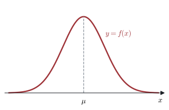
Properties of the normal curve Not in the formula booklet
- It is bell-shaped.
- It is symmetrical about the line \(x = \mu\), and it has one peak (it is unimodal).
- mean \(=\) median \(=\) mode \(= \mu\).
- The total area under the curve is \(1\).
- The curve gets closer and closer to the \(x\)-axis but never touches it (the \(x\)-axis is an asymptote).
- \(\mu\): the mean of the normal distribution
We write
\[ X \sim \mathrm{N}(\mu, \sigma^2) \]
to say that \(X\) is normal with mean \(\mu\) and variance \(\sigma^2\) (standard deviation \(\sigma\)). Careful: the second number is the variance. For example \(X \sim \mathrm{N}(20, 0.81)\) has \(\sigma = \sqrt{0.81} = 0.9\).
The probability density function (p.d.f.) of \(X \sim \mathrm{N}(\mu, \sigma^2)\) is
\[ f(x) = \frac{1}{\sigma\sqrt{2\pi}}\,\mathrm{e}^{-\frac{1}{2}\left(\frac{x - \mu}{\sigma}\right)^2}, \qquad x \in \mathbb{R} , \]
and \(\displaystyle\int_{-\infty}^{\infty} f(x)\,\mathrm{d}x = 1\). This integral cannot be done with the methods of this course, which is why we always use technology for normal probabilities. You do not need to learn this formula.
How \(\mu\) and \(\sigma\) change the curve
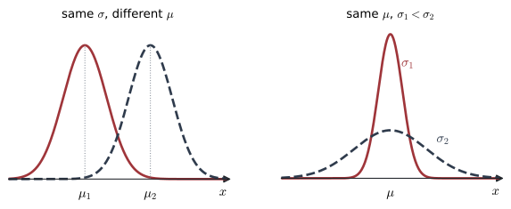
The shape of a normal curve is fixed by \(\mu\) and \(\sigma\).
- The mean \(\mu\) sets the position (the centre) of the curve.
- The standard deviation \(\sigma\) sets the spread. A larger \(\sigma\) gives a wider, lower curve; a smaller \(\sigma\) gives a narrow, tall curve. (The area is always \(1\), so a wider curve must be lower.)
The 68–95–99.7% rule
For every normal distribution, the area within \(k\) standard deviations of the mean is the same.
68–95–99.7% rule Not in the formula booklet
For \(X \sim \mathrm{N}(\mu, \sigma^2)\), approximately
- \(68\%\) of values lie between \(\mu - \sigma\) and \(\mu + \sigma\)
- \(95\%\) of values lie between \(\mu - 2\sigma\) and \(\mu + 2\sigma\)
- \(99.7\%\) of values lie between \(\mu - 3\sigma\) and \(\mu + 3\sigma\)
- \(X\): a normal random variable
- \(\mu\): the mean
- \(\sigma^2\): the variance
- \(\sigma\): the standard deviation
The syllabus expects you to know it.
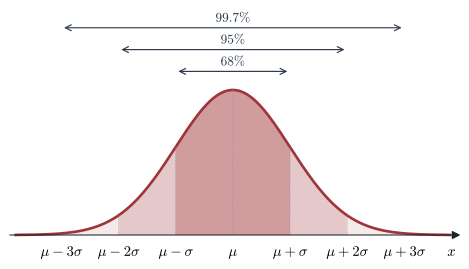
Use it with symmetry: each half of a band holds half of its percentage. For example, \(34\%\) lies between \(\mu\) and \(\mu + \sigma\), and \(2.5\%\) lies above \(\mu + 2\sigma\).
Example 1 The lengths, \(L\) mm, of leaves from a type of tree are normally distributed with mean \(80\) mm and standard deviation \(6\) mm. Without a calculator, estimate
(a) \(\mathrm{P}(74 < L < 86)\)
(b) \(\mathrm{P}(L > 92)\)
(c) \(\mathrm{P}(68 < L < 86)\)
(d) the number of leaves longer than \(86\) mm in a sample of \(400\) leaves.
Mark \(80 \pm 6\), \(80 \pm 12\), \(80 \pm 18\) on a sketch.
(a) \(74\) to \(86\) is \(\mu \pm \sigma\): about \(0.68\).
(b) \(92 = \mu + 2\sigma\). Outside \(\mu \pm 2\sigma\) is \(5\%\), half of it above: about \(0.025\).
(c) \(68 = \mu - 2\sigma\) and \(86 = \mu + \sigma\). Split at the mean: \(0.475 + 0.34 = 0.815\).
(d) \(\mathrm{P}(L > 86) \approx \dfrac{1 - 0.68}{2} = 0.16\), so about \(0.16 \times 400 = 64\) leaves.
The standard normal distribution
There are infinitely many normal distributions, one for each pair \(\mu, \sigma\). One of them is special.
Standard normal distribution Not in the formula booklet
If \(Z\) is normal with mean \(0\) and variance \(1\), we say \(Z\) has the standard normal distribution:
\[ Z \sim \mathrm{N}(0, 1) . \]
Before graphic display calculators, probabilities could not be calculated directly for a general \(\mathrm{N}(\mu, \sigma^2)\). Instead, every normal variable was changed into \(Z\) (see Section 19.4), and one printed table for \(Z\) was used. Today the GDC works with any \(\mu\) and \(\sigma\), but \(Z\) is still important for finding an unknown \(\mu\) or \(\sigma\).
\[ f(z) = \frac{1}{\sqrt{2\pi}}\,\mathrm{e}^{-\frac{1}{2}z^2}, \qquad z \in \mathbb{R} . \]
It has no parameters. On the TI-Nspire it is normPdf(z,0,1).
Cumulative probabilities
The cumulative distribution function of \(Z\) gives the area to the left of \(z\):
\[ \mathrm{P}(Z \leq z) = \int_{-\infty}^{z} f(t)\,\mathrm{d}t . \]
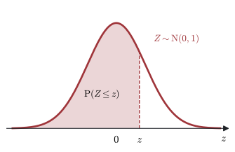
Because the curve is symmetrical about \(0\) and the total area is \(1\):
Useful facts for \(Z \sim \mathrm{N}(0, 1)\) (and \(a > 0\)) Not in the formula booklet
\[ \begin{aligned} \mathrm{P}(Z > a) &= 1 - \mathrm{P}(Z < a), \\ \mathrm{P}(Z < -a) &= \mathrm{P}(Z > a), \\ \mathrm{P}(-a < Z < a) &= 2\,\mathrm{P}(Z < a) - 1 . \end{aligned} \]
The same ideas work for any \(X \sim \mathrm{N}(\mu, \sigma^2)\), using symmetry about \(\mu\).
- \(Z\): a standard normal random variable
- \(a\): a positive constant
- \(X\): any normal random variable
- \(\mu\): the mean of \(X\)
- \(\sigma^2\): the variance of \(X\)
Normal probability calculations
The syllabus says that normal probabilities must be found using technology. Always draw a quick sketch with the mean and the required region shaded. It helps you to check that the answer is sensible.
Example 2 The heights of adult women in a town are normally distributed with mean \(165\) cm and standard deviation \(7\) cm. Find the probability that a woman chosen at random has height
(a) between \(155\) cm and \(168\) cm,
(b) less than \(175\) cm,
(c) more than \(162\) cm,
(d) within two standard deviations of the mean.
Let \(H \sim \mathrm{N}(165, 7^2)\).
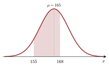
(a) normCdf(155,168,165,7) \(= 0.589\) (3 s.f.).
(b) \(\mathrm{P}(H < 175)\): normCdf(-1E99,175,165,7) \(= 0.923\).
(c) \(\mathrm{P}(H > 162)\): normCdf(162,1E99,165,7) \(= 0.666\). (Sensible: \(162\) is below the mean, so the answer is more than \(0.5\).)
(d) \(165 \pm 2 \times 7\), so \(\mathrm{P}(151 < H < 179)\): normCdf(151,179,165,7) \(= 0.954\). This agrees with the “95%” of the 68–95–99.7% rule.
Inverse normal calculations
In an inverse problem we know a probability (an area) and want the value of \(x\). The GDC command Inverse Normal (invNorm) takes the area to the left of \(x\).
Inverse normal
If \(\mathrm{P}(X < x) = p\), then \(x = \mathtt{invNorm}(p, \mu, \sigma)\).
If you are given a right-hand area, change it first: \(\mathrm{P}(X > x) = p \iff \mathrm{P}(X < x) = 1 - p\).
- \(X\): a normal random variable, \(X \sim \mathrm{N}(\mu, \sigma^2)\)
- \(x\): the value we want to find
- \(p\): the given probability (an area)
- \(\mu\): the mean of \(X\)
- \(\sigma\): the standard deviation of \(X\)
In SL 4.9, \(\mu\) and \(\sigma\) are given, and you do not need to change to \(Z\). (Unknown \(\mu\) or \(\sigma\) is in Section 19.4.)
Example 3 Given \(Z \sim \mathrm{N}(0, 1)\), find the value of \(a\), to three decimal places, for which
(a) \(\mathrm{P}(Z \leq a) = 0.95\)
(b) \(\mathrm{P}(|Z| < a) = 0.4\)
(a) invNorm(0.95,0,1) \(= 1.645\).
(b) \(|Z| < a\) means \(-a < Z < a\). This central area is \(0.4\), so each tail has area \(\dfrac{1 - 0.4}{2} = 0.3\). Then \(\mathrm{P}(Z < a) = 0.4 + 0.3 = 0.7\):
\[ a = \mathtt{invNorm}(0.7, 0, 1) = 0.524 . \]
Example 4 Given that \(X \sim \mathrm{N}(20, 0.81)\), find the value of
(a) \(m\) if \(\mathrm{P}(X > m) = 0.3\),
(b) \(w\) if \(\mathrm{P}(w < X < 21.2) = 0.58\),
(c) \(r\) if \(\mathrm{P}(X > r) \leq 0.4\).
\(\sigma = \sqrt{0.81} = 0.9\) (not \(0.81\)).
(a) The area to the left of \(m\) is \(1 - 0.3 = 0.7\).
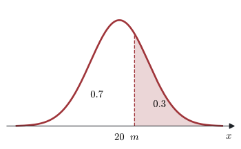
\[ m = \mathtt{invNorm}(0.7, 20, 0.9) = 20.5 \text{ (3 s.f.)} . \]
(b) First, \(\mathrm{P}(X < 21.2) = \mathtt{normCdf}(-\infty, 21.2, 20, 0.9) = 0.90879\ldots\) Then
\[ \mathrm{P}(X < w) = \mathrm{P}(X < 21.2) - \mathrm{P}(w < X < 21.2) = 0.90879\ldots - 0.58 = 0.32879\ldots \]
\[ w = \mathtt{invNorm}(0.32879\ldots, 20, 0.9) = 19.6 \text{ (3 s.f.)} . \]
(c) \(\mathrm{P}(X > r) = 0.4\) when \(\mathrm{P}(X < r) = 0.6\), that is, \(r = \mathtt{invNorm}(0.6, 20, 0.9) = 20.228\ldots\) As \(r\) increases, the right-hand area \(\mathrm{P}(X > r)\) decreases. So \(\mathrm{P}(X > r) \leq 0.4\) when
\[ r \geq 20.2 \text{ (3 s.f.)} . \]
Using your GDC
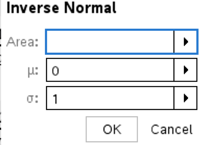
Calculator page → Menu → Probability → Distributions, then choose a command. Fill in the box and press OK.
| Command | Fields to fill in | What it gives | On the screen |
|---|---|---|---|
| Normal Cdf | Lower Bound, Upper Bound, \(\mu\), \(\sigma\) | \(\mathrm{P}(\text{lower} < X < \text{upper})\) | normCdf(lower, upper, μ, σ) |
| Inverse Normal | Area, \(\mu\), \(\sigma\) | the \(x\) with area to its left equal to Area | invNorm(area, μ, σ) |
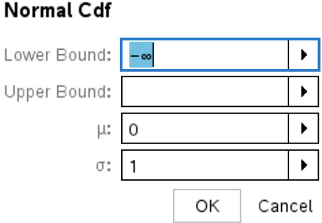
- The Lower Bound of Normal Cdf starts at \(-\infty\). So for “less than \(b\)” you only type the Upper Bound.
- For “more than \(a\)”, type \(a\) as the Lower Bound and a very large Upper Bound,
1E99(the EE key givesE). When you type the command yourself, \(-\infty\) can be written-1E99. - \(\mu\) and \(\sigma\) start at \(0\) and \(1\) (the standard normal). Change them for \(\mathrm{N}(\mu, \sigma^2)\).
- Normal Pdf gives only the height of the curve, not a probability. It is useful only for drawing the curve in a Graphs page: \(f_1(x) = \texttt{normPdf}(x, \mu, \sigma)\).
- Enter the standard deviation \(\sigma\), not the variance \(\sigma^2\).
- The Inverse Normal box always uses the area to the left. For an area to the right, type \(1 -\) (that area).
- Keep full accuracy in the calculator (store values, or use ans) and round only the final answer, to 3 s.f.
Common errors
| ✗ Wrong | ✓ Right | Why |
|---|---|---|
| \(\mathrm{N}(20, 0.81)\): entering \(\sigma = 0.81\) | \(\sigma = \sqrt{0.81} = 0.9\) | The second number in \(\mathrm{N}(\mu, \sigma^2)\) is the variance. |
| \(\mathrm{P}(X > m) = 0.3 \Rightarrow m = \mathtt{invNorm}(0.3, \ldots)\) | \(m = \mathtt{invNorm}(0.7, \ldots)\) | invNorm uses the area to the left. |
Using normPdf for a probability |
Use normCdf |
normPdf gives the height of the curve. |
| \(\mathrm{P}(\lvert Z\rvert < a) = 0.4 \Rightarrow a = \mathtt{invNorm}(0.4)\) | \(a = \mathtt{invNorm}(0.7)\) | Add the left tail \(0.3\) to the central \(0.4\). |
| A probability above \(0.5\) for a region far from the mean | Sketch first | A sketch quickly shows if an answer is impossible. |
| Rounding \(\mathrm{P}(X < 21.2)\) to \(0.91\) before subtracting | Keep full accuracy | Early rounding changes the final answer. |
Exercises
1 Paper 1 \(X \sim \mathrm{N}(50, 4^2)\). Use the 68–95–99.7% rule to estimate
(a) \(\mathrm{P}(46 < X < 54)\)
(b) \(\mathrm{P}(X > 58)\)
(c) \(\mathrm{P}(42 < X < 54)\).
(a) \(\mu \pm \sigma\): \(0.68\).
(b) \(58 = \mu + 2\sigma\): \(\dfrac{1 - 0.95}{2} = 0.025\).
(c) \(0.475 + 0.34 = 0.815\).
2 Paper 1 \(X \sim \mathrm{N}(10, \sigma^2)\) and \(\mathrm{P}(X > 12) = 0.2\). Write down
(a) \(\mathrm{P}(X < 8)\)
(b) \(\mathrm{P}(8 < X < 12)\)
(c) \(\mathrm{P}(10 < X < 12)\).
\(8\) and \(12\) are the same distance from \(\mu = 10\).
(a) By symmetry, \(0.2\).
(b) \(1 - 0.2 - 0.2 = 0.6\).
(c) \(0.5 - 0.2 = 0.3\).
3 \(Z \sim \mathrm{N}(0, 1)\). Find
(a) \(\mathrm{P}(Z < 1.2)\)
(b) \(\mathrm{P}(Z > -0.8)\)
(c) \(\mathrm{P}(-1.5 < Z < 0.5)\).
(a) \(0.885\) \(\quad\) (b) \(0.788\) \(\quad\) (c) \(0.625\) (all 3 s.f.).
4 \(X \sim \mathrm{N}(20, 9)\). Find
(a) \(\mathrm{P}(X < 25)\)
(b) \(\mathrm{P}(X > 17.5)\)
(c) \(\mathrm{P}(18 < X < 24)\).
\(\sigma = 3\).
(a) normCdf(-1E99,25,20,3) \(= 0.952\).
(b) normCdf(17.5,1E99,20,3) \(= 0.798\).
(c) normCdf(18,24,20,3) \(= 0.656\).
5 The lengths of bolts are normally distributed with mean \(40\) mm and standard deviation \(0.5\) mm.
(a) Find the probability that a bolt is longer than \(41\) mm.
(b) In a box of \(500\) bolts, find the expected number with lengths between \(39.5\) mm and \(40.8\) mm.
(a) normCdf(41,1E99,40,0.5) \(= 0.0228\) (3 s.f.).
(b) normCdf(39.5,40.8,40,0.5) \(= 0.78655\ldots\), and \(500 \times 0.78655\ldots = 393.3\). About \(393\) bolts.
6 \(Z \sim \mathrm{N}(0, 1)\). Find \(a\), to 3 decimal places, if
(a) \(\mathrm{P}(Z < a) = 0.85\)
(b) \(\mathrm{P}(Z > a) = 0.1\)
(c) \(\mathrm{P}(|Z| < a) = 0.9\).
(a) invNorm(0.85) \(= 1.036\).
(b) invNorm(0.9) \(= 1.282\).
(c) \(\mathrm{P}(Z < a) = 0.95\), so \(a = 1.645\).
7 \(X \sim \mathrm{N}(70, 12^2)\). Find \(k\) if
(a) \(\mathrm{P}(X < k) = 0.2\)
(b) \(\mathrm{P}(X > k) = 0.05\).
(a) invNorm(0.2,70,12) \(= 59.9\).
(b) invNorm(0.95,70,12) \(= 89.7\).
8 \(X \sim \mathrm{N}(5, 0.04)\). Find \(d\) such that \(\mathrm{P}(5 - d < X < 5 + d) = 0.95\).
\(\sigma = 0.2\). The interval is symmetrical about the mean, so \(\mathrm{P}(X < 5 + d) = 0.975\).
\(5 + d = \mathtt{invNorm}(0.975, 5, 0.2) = 5.39199\ldots\), so \(d = 0.392\) (3 s.f.).
9 The time taken to complete a puzzle is normally distributed with mean \(32\) minutes and standard deviation \(5\) minutes. \(75\%\) of people take longer than \(t\) minutes. Find \(t\).
\(\mathrm{P}(T > t) = 0.75\), so \(\mathrm{P}(T < t) = 0.25\). \(\;t = \mathtt{invNorm}(0.25, 32, 5) = 28.6\) minutes.
10 \(X \sim \mathrm{N}(100, 15^2)\). Find the largest value of \(c\) for which \(\mathrm{P}(X > c) \geq 0.9\).
\(\mathrm{P}(X > c) = 0.9\) when \(c = \mathtt{invNorm}(0.1, 100, 15) = 80.776\ldots\) As \(c\) decreases, \(\mathrm{P}(X > c)\) increases. So we need \(c \leq 80.8\), and the largest value is \(c = 80.8\) (3 s.f.).