17.3 Making Predictions

SL 4.4 SL 4.10

In this section you will learn

how to use a regression line to estimate (predict) a value
the difference between interpolation and extrapolation
how to decide whether a prediction is reliable
why you need the $x$ on $y$ line to predict $x$ from a value of $y$
how to use the mean point to find missing data
(Extension) how a sine model can describe periodic data

Estimating values with a linear model

Once we have a regression line, we can substitute a value of one variable to estimate the other.

To estimate $y$ from a given $x$, use the regression line of $y$ on $x$.
To estimate $x$ from a given $y$, use the regression line of $x$ on $y$ (see Section 17.2).

Interpolation and extrapolation

Interpolation and extrapolation Not in the formula booklet

Interpolation: estimating a value inside the range of the data. If the correlation is strong, the estimate is usually reliable.
Extrapolation: estimating a value outside the range of the data. This is not reliable, even when $r$ is close to $\pm 1$, because the linear pattern may not continue outside the data.

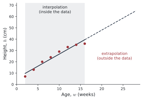
Figure 1: A line can fit well inside the data, but we cannot be sure it continues outside

In Figure 1 the plant heights already level off at the end of the data. The dashed part of the line keeps rising, so a prediction for 26 weeks would almost certainly be too large.

When is an estimate reliable?

An estimate from a regression line is reliable when

it is an interpolation (the given value is inside the range of the data), and
the correlation is strong ($\lvert r \rvert$ close to $1$), and
the correct line is used ($y$ on $x$ to find $y$; $x$ on $y$ to find $x$).

Example 1 For 15 young trees of the same type, aged between 2 and 12 years, the regression line of height ($y$ m) on age ($x$ years) is $y = 0.48x + 0.62$. The correlation coefficient is $r = 0.95$.

(a) Estimate the height of a tree that is 7 years old. Comment on the reliability of your estimate.

(b) Use the line to predict the height of a tree that is 60 years old. Comment on your answer.

Solution

(a) $y = 0.48 \times 7 + 0.62 = 3.98$ m. This is reliable: $x = 7$ is inside the data range ($2$ to $12$ years), and $r = 0.95$ shows strong positive correlation.

(b) $y = 0.48 \times 60 + 0.62 = 29.42$, about $29.4$ m. This is extrapolation: $60$ is far outside the range $2$ to $12$. Trees do not keep growing at a constant rate, so this prediction is not reliable, even though $r$ is high.

Example 2 A street stall records the maximum temperature ($T$ °C) and the number of iced drinks sold ($n$) on 10 days.

$T$	26.5	27.2	28.0	28.4	29.1	29.8	30.3	31.0	31.6	32.4
$n$	62	70	75	81	83	95	98	104	110	121

(a) Write down

(i) the mean temperature and the mean number of drinks sold;

(ii) the standard deviation of each variable.

(b) The regression line of $n$ on $T$ is $n = dT - 195$.

(i) Write down the value of $d$.

(ii) Estimate the number of drinks sold on a day when the maximum temperature is 29.6 °C.

(iii) Interpret the value of $d$.

(iv) Show that the mean point lies on the regression line.

Solution

(a) One-variable statistics on the GDC:

(i) $\bar{T} = 29.43 \approx 29.4$ °C and $\bar{n} = 89.9$ drinks.

(ii) $\sigma_T = 1.83$ °C and $\sigma_n = 17.8$ drinks (3 s.f.).

(b)

(i) Linear Regression (mx+b) gives $m = 9.6827\ldots$ and $b = -195.06\ldots$, so $d = 9.68$ (3 s.f.).

(ii) $n = 9.6827\ldots \times 29.6 - 195.06\ldots = 91.5\ldots$, so about $92$ drinks. (This is interpolation and $r = 0.995$, so it is reliable.)

(iii) For each $1$ °C rise in temperature, the stall sells about $9.68$ more iced drinks, on average.

(iv) $9.68 \times 29.43 - 195 = 89.9$ (3 s.f.) $= \bar{n}$. So $(\bar{T}, \bar{n})$ lies on the line.

Predicting $x$ from a value of $y$

SL 4.10

A $y$ on $x$ line is designed to predict $y$. If you rearrange it to find $x$ from $y$, the answer is in general not the best estimate.

Which line for which prediction?

Given $x$, estimate $y$: use the $y$ on $x$ line.
Given $y$, estimate $x$: use the $x$ on $y$ line.
If $x$ is a controlled variable, only the $y$ on $x$ line makes sense. Then you cannot reliably predict $x$ from $y$.

Example 3 The masses ($x$ kg) and heights ($y$ cm) of 25 ten-year-old children were measured. Neither variable was controlled. The masses were between $28$ and $47$ kg and the heights between $125$ and $152$ cm. $r = 0.812$.

Regression line of $y$ on $x$: $\;y = 1.2x + 94.8$. $\qquad$ Regression line of $x$ on $y$: $\;x = 0.55y - 39.9$.

(a) Estimate the height of a child with a mass of $40$ kg.

(b) Estimate the mass of a child with a height of $150$ cm.

(c) Find the mean mass and the mean height of the children.

Solution

(a) Given $x$, use $y$ on $x$: $\;y = 1.2 \times 40 + 94.8 = 142.8$ cm.

(b) Given $y$, use $x$ on $y$: $\;x = 0.55 \times 150 - 39.9 = 42.6$ kg.

(Rearranging the $y$ on $x$ line would give $x = \dfrac{150 - 94.8}{1.2} = 46$ kg — a different, wrong estimate.)

(c) Both lines pass through $(\bar{x}, \bar{y})$:

\[ x = 0.55(1.2x + 94.8) - 39.9 = 0.66x + 12.24 \;\Longrightarrow\; 0.34x = 12.24 \;\Longrightarrow\; x = 36 . \]

$y = 1.2 \times 36 + 94.8 = 138$. The mean mass is $36$ kg and the mean height is $138$ cm.

Using the mean point to find missing data

The regression line passes through $(\bar{x}, \bar{y})$. So if one data value is unknown, you can find $\bar{y}$ from the line, and then the total $\sum y = n\bar{y}$. This works without a calculator.

Example 4 The height ($h$ cm) of a plant was measured every two weeks ($w$ = age in weeks). One value is missing.

$w$	2	4	6	8	10	12	14	16
$h$	7	13	20	24	$k$	33	35	36

(a) The regression line of $h$ on $w$ is $h = 2.125w + 5.5$. Find $k$.

(b) Interpret the gradient of the line.

(c) Use the line to estimate the height at $w = 30$ weeks, and comment on your answer.

Solution

(a) $\bar{w} = \dfrac{72}{8} = 9$. The line passes through $(\bar{w}, \bar{h})$:

\[ \bar{h} = 2.125 \times 9 + 5.5 = 24.625 . \]

So $\sum h = 8 \times 24.625 = 197$. The known values add to $7 + 13 + 20 + 24 + 33 + 35 + 36 = 168$, so

\[ k = 197 - 168 = 29 . \]

(b) On average, the plant grows about $2.1$ cm per week (between 2 and 16 weeks).

(c) $h = 2.125 \times 30 + 5.5 = 69.25 \approx 69$ cm. This is extrapolation ($30 > 16$). The data shows the growth slowing down (only $1$ cm between weeks 14 and 16), so the estimate is not reliable and is probably much too large. See Figure 1.

Example 5 A laboratory measures the area ($y$ cm²) covered by a mould at fixed times ($x$ days).

$x$	4	9	15	22	30	38	45
$y$	3.2	9.8	51.6	21.5	30.4	40.8	47.9

(a) One of the results is probably wrong. Identify it and explain your answer.

(b) The wrong result is corrected. For the corrected data the two regression lines are

\[ y = 1.07723x - 0.912562 \qquad\text{and}\qquad x = 0.925660y + 0.911183 . \]

(i) Find the corrected value, to 1 decimal place.

(ii) State, with a reason, which line should be used to model the relationship.

(iii) Use your line to estimate the area after 26 days, and comment on the reliability.

Solution

(a) $y = 51.6$ at $x = 15$. The other values increase steadily, but $51.6$ is much larger than the value at $x = 22$ and even larger than the value at $x = 45$. It does not fit the pattern. (It may be $15.6$ with the digits swapped.)

(b)

(i) Both lines pass through $(\bar{x}, \bar{y})$, and $\bar{x} = \dfrac{163}{7}$. From the $y$ on $x$ line:

\[ \bar{y} = 1.07723 \times \frac{163}{7} - 0.912562 = 24.1715\ldots \]

(We know $\bar{x}$ exactly, so we do not need to solve the two equations together. The two lines are almost parallel here, so solving them would magnify rounding errors.) So $\sum y = 7 \times 24.1715\ldots = 169.20\ldots$. The six correct values add to $3.2 + 9.8 + 21.5 + 30.4 + 40.8 + 47.9 = 153.6$, so the corrected value is

\[ 169.2 - 153.6 = 15.6 . \]

(ii) The time $x$ is fixed by the laboratory, so $x$ is the independent variable. Use the regression line of $y$ on $x$.

(iii) $y = 1.07723 \times 26 - 0.912562 = 27.1$ cm² (3 s.f.). This is reliable: $26$ is inside the data range ($4$ to $45$ days), and the correlation is very strong ($r = 0.999$ for the corrected data).

Extension Periodic data and sine models

Extension — modelling periodic data with a sine function (needs Unit 14)

Regression is not only for straight lines. A GDC can also fit curves, for example exponential or polynomial models. These are not in the AA syllabus. But some real data repeats in cycles (temperatures over a year, tide heights, hours of daylight). Such data can often be modelled by

\[ y = a\sin\big(b(x - c)\big) + d . \]

You need the properties of sine graphs from Unit 14 (amplitude, period, horizontal and vertical shift). You can estimate $a$, $b$, $c$ and $d$ by hand and then check your model with SinReg on the GDC.

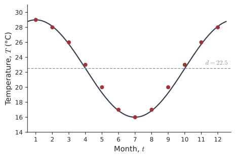
Example 6 The mean monthly maximum temperature ($T$ °C) in a city in the southern hemisphere is shown ($t = 1$ is January).

$t$	1	2	3	4	5	6	7	8	9	10	11	12
$T$	29	28	26	23	20	17	16	17	20	23	26	28

(a) Why is a trigonometric model suitable?

(b) Without technology, find values of $a$, $b$, $c$ and $d$ for a model $T = a\sin\big(b(t - c)\big) + d$.

(c) Compare your model with the GDC’s sinusoidal regression.

Solution

(a) The temperatures fall and then rise again, and the pattern will repeat every 12 months. The data is periodic.

(b) Maximum $29$ (at $t = 1$), minimum $16$ (at $t = 7$).

$d = \dfrac{29 + 16}{2} = 22.5$ (the principal axis).
$a = \dfrac{29 - 16}{2} = 6.5$ (the amplitude).
The period is $12$ months, so $b = \dfrac{2\pi}{12} = \dfrac{\pi}{6} \approx 0.524$.
A sine curve with $a > 0$ crosses its axis going up at $t = c$. The temperature rises through $22.5$ halfway between the minimum ($t = 7$) and the next maximum ($t = 13$), so $c = 10$.

\[ T = 6.5\sin\left(\frac{\pi}{6}(t - 10)\right) + 22.5 \]

(c) Lists & Spreadsheet → Menu → Statistics → Stat Calculations → Sinusoidal Regression. Written in the same form, the GDC gives about $T = 6.25\sin\big(0.545(t - 9.88)\big) + 22.5$, which is very close to our model. Every value of our model is within $0.75$ °C of the data, so the model fits well.

Figure 2: The data and the model $T = 6.5\sin\left(\frac{\pi}{6}(t - 10)\right) + 22.5$

Using your GDC

Task	TI-Nspire CX II
Find the line	Lists & Spreadsheet → Menu → Statistics → Stat Calculations → Linear Regression (mx+b). Tick Save RegEqn to: `f1`.
Predict $y$ from $x$	On a Calculator page type `f1(29.6)` — this uses the unrounded coefficients.
Predict $x$ from $y$	Run the regression again with the lists swapped, save to `f2`, then type `f2(150)`.
Mean point	One-Variable Statistics on each list, or solve the two regression equations.

Common errors

✗ Wrong	✓ Right	Why
“$r = 0.99$, so the prediction for $x = 60$ is reliable.”	It is extrapolation, so it is not reliable.	The pattern may change outside the data.
“$x = 12$ is inside the data, so the estimate is reliable.” (with $r = 0.21$)	Not reliable.	The correlation must also be strong.
Rearranging the $y$ on $x$ line to find $x$	Use the $x$ on $y$ line	The $y$ on $x$ line is not designed to predict $x$.
Predicting $x$ from $y$ when $x$ is controlled	Say it cannot be done reliably	Only the $y$ on $x$ line makes sense then.
Accepting a negative price, length or time	Comment that the value is impossible	A sign that the model has been used outside its range.
Using rounded coefficients in a long calculation	Use the stored GDC values	Rounding errors can change the final answer.

Exercises

1 A regression line was found from data with $15 \le x \le 60$. State whether each estimate is interpolation or extrapolation.

(a) $x = 20$

(b) $x = 75$

(c) $x = 59$

(d) $x = 5$

Solution

(a) interpolation

(b) extrapolation

(c) interpolation

(d) extrapolation

2 Paper 1 For 15 car journeys of lengths $20$ to $180$ km, the regression line of fuel used ($y$ litres) on distance ($x$ km) is $y = 0.071x + 0.85$, with $r = 0.97$.

(a) Estimate the fuel used on a 100 km journey and comment on the reliability.

(b) Estimate the fuel used on a 400 km journey and comment.

Solution

(a) $y = 0.071 \times 100 + 0.85 = 7.95$ litres. Reliable: inside the data and $r$ is strong.

(b) $y = 0.071 \times 400 + 0.85 = 29.25$ litres. Not reliable: $400$ km is outside the data (extrapolation). Long journeys may use mostly motorways, where fuel use per km is different.

3 Paper 2 The age of a laptop battery ($x$ months) and its running time on a full charge ($y$ hours) are shown.

$x$	3	6	9	12	15	18	21	24
$y$	9.8	9.5	9.1	8.6	8.4	7.9	7.6	7.1

(a) Find $r$ and the regression line of $y$ on $x$.

(b) Estimate the running time after 10 months.

(c) Use the line to estimate the running time after 100 months, and comment.

Solution

(a) $r = -0.998$; $\;y = -0.128x + 10.2$ (3 s.f.).

(b) $y = 8.95$ hours (3 s.f., using the full GDC values).

(c) $y = -2.55$ hours. A negative running time is impossible. $100$ months is far outside the data, so the line should not be used there.

4 Paper 1 For 20 students, the regression line of French score ($y$) on English score ($x$) is $y = 0.72x + 11.8$, and the regression line of $x$ on $y$ is $x = 0.95y + 7.75$.

(a) Estimate the French score of a student who scored $70$ in English.

(b) Estimate the English score of a student who scored $48$ in French.

(c) Find the mean English score and the mean French score.

Solution

(a) $y = 0.72 \times 70 + 11.8 = 62.2$, about $62$.

(b) Use $x$ on $y$: $x = 0.95 \times 48 + 7.75 = 53.35$, about $53$.

(c) $x = 0.95(0.72x + 11.8) + 7.75 = 0.684x + 18.96 \Rightarrow 0.316x = 18.96 \Rightarrow x = 60$. Then $y = 0.72 \times 60 + 11.8 = 55$. Mean English score $60$, mean French score $55$.

5 Paper 1 The regression line of $y$ on $x$ for the data below is $y = 1.95x + 1.1$. Find $k$.

$x$	2	4	6	8	10
$y$	5	9	$k$	16	21

Solution

$\bar{x} = 6$, so $\bar{y} = 1.95 \times 6 + 1.1 = 12.8$ and $\sum y = 5 \times 12.8 = 64$.

$k = 64 - (5 + 9 + 16 + 21) = 64 - 51 = 13$.

6 For data with $5 \le x \le 25$, the regression line of $y$ on $x$ is $y = 2.4x + 30$ and $r = 0.21$. A student estimates $y$ when $x = 12$ and says the answer is reliable because $12$ is inside the data. Comment.

Solution

The estimate is $y = 2.4 \times 12 + 30 = 58.8$, but it is not reliable. $r = 0.21$ shows very weak correlation, so the points are far from the line. An estimate must be inside the data and have strong correlation.

7 Paper 1 For cars between 1 and 8 years old, the regression line of value ($V$ thousand dollars) on age ($t$ years) is $V = -2.15t + 24.3$.

(a) Interpret the value $-2.15$.

(b) Estimate the value of a 5-year-old car.

(c) Find the value predicted for a 15-year-old car and comment.

Solution

(a) On average, the value falls by about $2150 each year.

(b) $V = -2.15 \times 5 + 24.3 = 13.55$, about $13 550.

(c) $V = -2.15 \times 15 + 24.3 = -7.95$. A negative value is impossible. $t = 15$ is outside the data, so the linear model does not apply.

8 Paper 2 Seven pairs of data are shown.

$x$	10	20	30	40	50	60	70
$y$	15	24	36	44	13	63	75

(a) Identify the result that is probably wrong.

(b) Remove it, and find the regression line of $y$ on $x$ for the other six points.

(c) Estimate the correct value of $y$ when $x = 50$.

Solution

(a) $(50, 13)$: all the other $y$-values increase steadily with $x$.

(b) GDC: $y = 0.987x + 5.00$ (3 s.f.), with $r = 0.999$.

(c) $y = 0.98695\ldots \times 50 + 5.00 = 54.3$ (3 s.f.).

9 Paper 1 For data with $5 \le x \le 20$, $\bar{x} = 12.5$ and $\bar{y} = 40.2$. The regression line of $y$ on $x$ has gradient $2.6$.

(a) Find the equation of the line.

(b) Estimate $y$ when $x = 15$.

Solution

(a) $40.2 = 2.6 \times 12.5 + b \Rightarrow b = 40.2 - 32.5 = 7.7$. So $y = 2.6x + 7.7$.

(b) $y = 2.6 \times 15 + 7.7 = 46.7$.

10 Paper 2 The distance from a city centre ($x$ km) and the price of flats ($y$ thousand dollars per m²) are recorded for eight areas.

$x$	1	2	4	5	7	8	10	12
$y$	14.2	13.1	12.0	11.2	9.6	9.4	7.5	6.1

(a) Find $r$ and describe the correlation.

(b) Find the regression line of $y$ on $x$, and interpret its gradient.

(c) Estimate the price at $6$ km from the centre.

(d) Estimate the price at $30$ km from the centre and comment.

Solution

(a) $r = -0.998$: very strong negative linear correlation.

(b) $y = -0.719x + 14.8$ (3 s.f.). The price falls by about $719 per m² for each extra kilometre from the centre.

(c) $y = 10.5$ thousand dollars per m² (3 s.f.). Reliable: interpolation with strong correlation.

(d) $y = -6.78$. A negative price is impossible: $30$ km is far outside the data, so this extrapolation is meaningless.

Estimating values with a linear model

Interpolation and extrapolation

Predicting \(x\) from a value of \(y\)

Using the mean point to find missing data

Extension Periodic data and sine models

Using your GDC

Common errors

Exercises