19.2 Variance, Mode and Median of a Continuous Random Variable
AHL 4.14
- how to find the variance \(\mathrm{Var}(X) = \mathrm{E}(X^2) - \big(\mathrm{E}(X)\big)^2\) and the standard deviation of a continuous random variable
- the effect of a linear transformation: \(\mathrm{Var}(aX + b) = a^2\,\mathrm{Var}(X)\)
- how to find the expected value and variance of a function of \(X\)
- how to find the mode (where \(f(x)\) is greatest) and the median \(m\), where \(\displaystyle\int_{-\infty}^{m} f(x)\,\mathrm{d}x = \frac{1}{2}\)
- (Extension) percentiles and quartiles of a continuous random variable
Variance
For any random variable \(X\) (discrete or continuous) with mean \(\mu = \mathrm{E}(X)\), the variance is
\[ \mathrm{Var}(X) = \mathrm{E}\big((X - \mu)^2\big) , \]
the mean of the squared distance from the mean. A shorter way to calculate it uses the rules of Section 19.1:
\[ \begin{aligned} \mathrm{E}\big((X - \mu)^2\big) &= \mathrm{E}(X^2 - 2\mu X + \mu^2) \\ &= \mathrm{E}(X^2) - 2\mu\,\mathrm{E}(X) + \mu^2 \\ &= \mathrm{E}(X^2) - 2\mu^2 + \mu^2 \\ &= \mathrm{E}(X^2) - \mu^2 . \end{aligned} \]
Variance of a continuous random variable In the HL formula booklet
\[ \mathrm{Var}(X) = \int_{-\infty}^{\infty} (x - \mu)^2 f(x)\,\mathrm{d}x = \int_{-\infty}^{\infty} x^2 f(x)\,\mathrm{d}x - \mu^2 \]
\[ \mathrm{Var}(X) = \mathrm{E}\big[(X - \mu)^2\big] = \mathrm{E}(X^2) - [\mathrm{E}(X)]^2 \] where \[ \mathrm{E}(X^2) = \int_{-\infty}^{\infty} x^2 f(x)\,\mathrm{d}x . \]
- \(\mathrm{Var}(X)\): the variance of \(X\)
- \(x\): a value of \(X\) (the variable of integration)
- \(\mu\): the mean of \(X\), \(\mu = \mathrm{E}(X)\)
- \(f(x)\): the probability density function (p.d.f.) of \(X\)
- \(\mathrm{E}(X^2)\): the expected value of \(X^2\)
- \(\mathrm{Var}(X)\) is often written \(\sigma^2\).
- The standard deviation of \(X\) is \(\sigma = \sqrt{\mathrm{Var}(X)}\).
Variance and linear transformations Partly in the HL formula booklet
For constants \(a\) and \(b\):
\[ \mathrm{Var}(aX + b) = a^2\,\mathrm{Var}(X) \]
In the HL booklet
In particular,
\[ \mathrm{Var}(a) = 0, \qquad \mathrm{Var}(aX) = a^2\,\mathrm{Var}(X) . \]
Adding \(b\) moves the distribution but does not change its spread, so \(b\) disappears. Multiplying by \(a\) multiplies every distance from the mean by \(a\), so the variance is multiplied by \(a^2\) (and the standard deviation by \(|a|\)).
If \(X\) and \(Y\) are independent, then
\[ \mathrm{Var}(aX \pm bY) = a^2\,\mathrm{Var}(X) + b^2\,\mathrm{Var}(Y) . \]
Notice the plus sign in both cases: variances always add. This is not in the AA syllabus.
Example 1 The continuous random variable \(X\) has probability density function
\[ f(x) = \begin{cases} \dfrac{3}{8}(2 - x)^2, & 0 \leq x \leq 2 \\[2pt] 0, & \text{otherwise.} \end{cases} \]
(a) Find \(\mathrm{E}(X)\) and \(\mathrm{Var}(X)\).
(b) Given that \(\mathrm{E}(4X - c) = 1\), find the value of the constant \(c\).
(a) Expand: \((2 - x)^2 = 4 - 4x + x^2\).
\[ \mathrm{E}(X) = \frac{3}{8}\int_0^2 \left(4x - 4x^2 + x^3\right)\mathrm{d}x = \frac{3}{8}\left[2x^2 - \frac{4x^3}{3} + \frac{x^4}{4}\right]_0^2 = \frac{3}{8}\left(8 - \frac{32}{3} + 4\right) = \frac{3}{8} \times \frac{4}{3} = \frac{1}{2} . \]
\[ \begin{aligned} \mathrm{E}(X^2) &= \frac{3}{8}\int_0^2 \left(4x^2 - 4x^3 + x^4\right)\mathrm{d}x \\ &= \frac{3}{8}\left[\frac{4x^3}{3} - x^4 + \frac{x^5}{5}\right]_0^2 \\ &= \frac{3}{8}\left(\frac{32}{3} - 16 + \frac{32}{5}\right) \\ &= \frac{3}{8} \times \frac{16}{15} \\ &= \frac{2}{5} . \end{aligned} \]
\[ \mathrm{Var}(X) = \frac{2}{5} - \left(\frac{1}{2}\right)^2 = \frac{3}{20} . \]
(b) \(\mathrm{E}(4X - c) = 4\,\mathrm{E}(X) - c = 2 - c = 1\), so \(c = 1\).
Example 2 A continuous random variable \(X\) has probability density function
\[ f(x) = \begin{cases} \dfrac{x}{8}, & 0 \leq x \leq 2 \\[2pt] \dfrac{1}{4}, & 2 < x \leq 5 \\[2pt] 0, & \text{otherwise.} \end{cases} \]
(a) Sketch the graph of \(y = f(x)\).
(b) Find the mean \(\mu\) and the variance \(\sigma^2\).
(c) Find \(\mathrm{E}(2X - 5)\) and \(\mathrm{Var}(4X + 1)\).
(d) Find \(\mathrm{P}(|X - \mu| < \sigma)\).
(a) A straight line from \((0, 0)\) to \(\left(2, \frac{1}{4}\right)\), then a horizontal line to \(x = 5\).
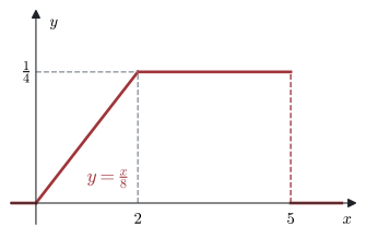
(Check: the areas are \(\frac{1}{2} \times 2 \times \frac{1}{4} = \frac{1}{4}\) and \(3 \times \frac{1}{4} = \frac{3}{4}\), total \(1\).)
(b) Split each integral at \(x = 2\):
\[ \mu = \int_0^2 \frac{x^2}{8}\,\mathrm{d}x + \int_2^5 \frac{x}{4}\,\mathrm{d}x = \frac{8}{24} + \frac{25 - 4}{8} = \frac{1}{3} + \frac{21}{8} = \frac{71}{24} \;(\approx 2.96) . \]
\[ \mathrm{E}(X^2) = \int_0^2 \frac{x^3}{8}\,\mathrm{d}x + \int_2^5 \frac{x^2}{4}\,\mathrm{d}x = \frac{16}{32} + \frac{125 - 8}{12} = \frac{1}{2} + \frac{39}{4} = \frac{41}{4} . \]
\[ \sigma^2 = \frac{41}{4} - \left(\frac{71}{24}\right)^2 = \frac{5904}{576} - \frac{5041}{576} = \frac{863}{576} \;(\approx 1.50) . \]
(c) \(\mathrm{E}(2X - 5) = 2 \times \dfrac{71}{24} - 5 = \dfrac{71}{12} - \dfrac{60}{12} = \dfrac{11}{12}\).
\(\mathrm{Var}(4X + 1) = 16 \times \dfrac{863}{576} = \dfrac{863}{36}\) \(\;(\approx 24.0)\).
(d) \(\sigma = \sqrt{\frac{863}{576}} = 1.2240\ldots\), so \(|X - \mu| < \sigma\) means
\[ \mu - \sigma < X < \mu + \sigma, \qquad\text{that is}\qquad 1.7343 < X < 4.1824 . \]
This interval crosses \(x = 2\), so split it:
\[ \begin{aligned} \mathrm{P}(|X - \mu| < \sigma) &= \int_{1.7343}^{2} \frac{x}{8}\,\mathrm{d}x + \int_2^{4.1824} \frac{1}{4}\,\mathrm{d}x \\ &= \frac{4 - 1.7343^2}{16} + \frac{2.1824}{4} \\ &= 0.0620 + 0.5456 = 0.608 \text{ (3 s.f.)} . \end{aligned} \]
Store the values first: m:=71/24 and s:=√(863/576). Then Menu → Calculus → Numerical Integral twice: \(\displaystyle\int_{m-s}^{2} \frac{x}{8}\,\mathrm{d}x + \int_{2}^{m+s} \frac{1}{4}\,\mathrm{d}x = 0.6076\ldots\) Keeping the stored values avoids rounding errors.
Expected value and variance of a function of \(X\)
If \(Y = g(X)\), use \(\mathrm{E}\big(g(X)\big) = \displaystyle\int g(x)\,f(x)\,\mathrm{d}x\) for \(\mathrm{E}(Y)\) and for \(\mathrm{E}(Y^2)\), then \(\mathrm{Var}(Y) = \mathrm{E}(Y^2) - \big(\mathrm{E}(Y)\big)^2\).
Example 3 The continuous random variable \(X\) has probability density function
\[ f(x) = \begin{cases} \dfrac{2}{3}(x + 1), & 0 \leq x \leq 1 \\[2pt] 0, & \text{otherwise.} \end{cases} \]
Find the expected value and the variance of \(Y\), where \(Y = \sqrt{X}\).
\[ \mathrm{E}(Y) = \int_0^1 \sqrt{x} \times \frac{2}{3}(x + 1)\,\mathrm{d}x = \frac{2}{3}\int_0^1 \left(x^{\frac{3}{2}} + x^{\frac{1}{2}}\right)\mathrm{d}x = \frac{2}{3}\left(\frac{2}{5} + \frac{2}{3}\right) = \frac{2}{3} \times \frac{16}{15} = \frac{32}{45} . \]
\(Y^2 = X\), so
\[ \mathrm{E}(Y^2) = \mathrm{E}(X) = \frac{2}{3}\int_0^1 \left(x^2 + x\right)\mathrm{d}x = \frac{2}{3}\left(\frac{1}{3} + \frac{1}{2}\right) = \frac{5}{9} . \]
\[ \mathrm{Var}(Y) = \frac{5}{9} - \left(\frac{32}{45}\right)^2 = \frac{1125}{2025} - \frac{1024}{2025} = \frac{101}{2025} \;(\approx 0.0499) . \]
Mode of a continuous random variable
Mode Not in the formula booklet
The mode of a continuous random variable \(X\) is the value of \(x\) at which the p.d.f. \(f(x)\) is greatest.
To find the mode:
- Sketch \(y = f(x)\). This shows where the maximum is. It may be at an end point of the interval.
- If the maximum is a turning point, solve \(f'(x) = 0\) (this needs \(f\) to be differentiable there), and check that it is a maximum.
Example 4 \(X\) has p.d.f. \(f(x) = \dfrac{1}{4}x(4 - x^2)\) for \(0 \leq x \leq 2\), and \(f(x) = 0\) otherwise. Find the mode of \(X\).
\(f(x) = x - \dfrac{x^3}{4}\), so \(f'(x) = 1 - \dfrac{3x^2}{4}\).
\[ f'(x) = 0 \;\Longrightarrow\; x^2 = \frac{4}{3} \;\Longrightarrow\; x = \frac{2}{\sqrt{3}} \;(\approx 1.15) \quad(\text{reject the negative root}). \]
\(f''(x) = -\dfrac{3x}{2} < 0\) for \(x > 0\), so this is a maximum. Also \(f(0) = f(2) = 0\), so the end points are not larger. The mode is \(\dfrac{2}{\sqrt{3}} = \dfrac{2\sqrt{3}}{3}\).
Median of a continuous random variable
Median Not in the formula booklet
The median \(m\) splits the total area under \(y = f(x)\) into two equal halves:
\[ \int_{-\infty}^{m} f(x)\,\mathrm{d}x = \frac{1}{2} . \]
If \(y = f(x)\) is symmetrical about \(x = c\), then the median is \(c\) (and the mean is also \(c\)).
- \(m\): the median of \(X\)
- \(f(x)\): the p.d.f. of \(X\)
- \(c\): a constant; \(x = c\) is the line of symmetry
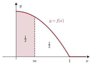
The median is the 50th percentile. In the same way:
- the \(p\)th percentile is the value \(t\) with \(\displaystyle\mathrm{P}(X \leq t) = \int_{-\infty}^{t} f(x)\,\mathrm{d}x = \frac{p}{100}\);
- the lower quartile \(q_1\) has \(\displaystyle\int_{-\infty}^{q_1} f(x)\,\mathrm{d}x = \frac{1}{4}\);
- the upper quartile \(q_3\) has \(\displaystyle\int_{-\infty}^{q_3} f(x)\,\mathrm{d}x = \frac{3}{4}\), or equivalently \(\mathrm{P}(X \geq q_3) = \dfrac{1}{4}\).
The IB syllabus names only the median, so percentiles and quartiles are marked Extension. They use exactly the same method.
Example 5 The continuous random variable \(X\) has probability density function
\[ f(x) = \begin{cases} \lambda\,\mathrm{e}^{-\frac{x}{3}}, & x \geq 0 \\ 0, & \text{otherwise.} \end{cases} \]
Find
(a) the value of \(\lambda\),
(b) the mode,
(c) the median,
(d) Extension the 20th percentile of \(X\).
(a) The interval goes to infinity, so take a limit:
\[ \int_0^{\infty} \lambda\,\mathrm{e}^{-\frac{x}{3}}\,\mathrm{d}x = \lim_{b \to \infty}\Big[-3\lambda\,\mathrm{e}^{-\frac{x}{3}}\Big]_0^{b} = \lim_{b \to \infty} 3\lambda\left(1 - \mathrm{e}^{-\frac{b}{3}}\right) = 3\lambda = 1 \;\Longrightarrow\; \lambda = \frac{1}{3} . \]
(b) \(f(x) = \dfrac{1}{3}\mathrm{e}^{-\frac{x}{3}}\) is decreasing for \(x \geq 0\), so its greatest value is at the end point \(x = 0\). The mode is \(0\).
(c) For \(t \geq 0\): \(\displaystyle\int_0^t \frac{1}{3}\mathrm{e}^{-\frac{x}{3}}\,\mathrm{d}x = 1 - \mathrm{e}^{-\frac{t}{3}}\).
\[ 1 - \mathrm{e}^{-\frac{m}{3}} = \frac{1}{2} \;\Longrightarrow\; \mathrm{e}^{-\frac{m}{3}} = \frac{1}{2} \;\Longrightarrow\; m = 3\ln 2 \;(\approx 2.08) . \]
(d) \(1 - \mathrm{e}^{-\frac{t}{3}} = 0.2 \Rightarrow \mathrm{e}^{-\frac{t}{3}} = 0.8 \Rightarrow t = -3\ln 0.8 = 3\ln\dfrac{5}{4} \;(\approx 0.669)\).
When the equation for \(m\) is a cubic (or worse), use your GDC.
Example 6 The continuous random variable \(X\) has probability density function
\[ f(x) = \begin{cases} \dfrac{3}{2}\left(1 - x^2\right), & 0 \leq x \leq 1 \\[2pt] 0, & \text{otherwise.} \end{cases} \]
Find the median of \(X\).
\[ \int_0^m \frac{3}{2}\left(1 - x^2\right)\mathrm{d}x = \frac{3}{2}\left(m - \frac{m^3}{3}\right) = \frac{1}{2} \;\Longrightarrow\; 3m - m^3 = 1 \;\Longrightarrow\; m^3 - 3m + 1 = 0 . \]
The median must be between \(0\) and \(1\). With a GDC, the root of \(m^3 - 3m + 1 = 0\) in \([0, 1]\) is
\[ m = 0.347 \text{ (3 s.f.)} . \]
(The cubic has two other roots, about \(1.53\) and \(-1.88\), but they are outside \([0, 1]\), so we reject them.)
Calculator page → Menu → Algebra → Numerical Solve:
nSolve( \(m^3 - 3m + 1 = 0,\ m\) )|0≤m≤1
The condition after | keeps the answer in the right interval. You can also solve \(\displaystyle\int_0^m \frac{3}{2}(1 - x^2)\,\mathrm{d}x = 0.5\) directly, without doing the integral by hand. Or graph \(y = x^3 - 3x + 1\) and use Menu → Analyze Graph → Zero.
Common errors
| ✗ Wrong | ✓ Right | Why |
|---|---|---|
| \(\mathrm{Var}(X) = \mathrm{E}(X^2)\) | \(\mathrm{Var}(X) = \mathrm{E}(X^2) - \mu^2\) | Do not forget to subtract \(\mu^2\). |
| \(\mathrm{Var}(4X + 1) = 4\,\mathrm{Var}(X) + 1\) | \(\mathrm{Var}(4X + 1) = 16\,\mathrm{Var}(X)\) | Square the multiplier; the added constant has no effect. |
| \(\mathrm{Var}(-2X) = -2\,\mathrm{Var}(X)\) | \(\mathrm{Var}(-2X) = 4\,\mathrm{Var}(X)\) | A variance is never negative. |
| Mode: solve \(f(x) = 0\) | Find where \(f(x)\) is greatest | Use \(f'(x) = 0\), or an end point. |
| Mode is always where \(f'(x) = 0\) | Check the end points too | In Example 5 the mode is the end point \(0\). |
| Median: \(\displaystyle\int_{-\infty}^{m} x\,f(x)\,\mathrm{d}x = \frac{1}{2}\) | \(\displaystyle\int_{-\infty}^{m} f(x)\,\mathrm{d}x = \frac{1}{2}\) | The median is about area (probability), not about \(x\,f(x)\). |
| Giving every root of the median equation | Choose the root inside the interval | \(f(x) = 0\) outside the interval. |
Exercises
1 \(X\) has p.d.f. \(f(x) = \dfrac{3}{8}x^2\) for \(0 \leq x \leq 2\), and \(f(x) = 0\) otherwise. Find \(\mathrm{Var}(X)\) and the standard deviation of \(X\).
\(\mathrm{E}(X) = \dfrac{3}{8} \times \dfrac{16}{4} = \dfrac{3}{2}\) and \(\mathrm{E}(X^2) = \dfrac{3}{8} \times \dfrac{32}{5} = \dfrac{12}{5}\).
\(\mathrm{Var}(X) = \dfrac{12}{5} - \dfrac{9}{4} = \dfrac{3}{20}\), and \(\sigma = \sqrt{\dfrac{3}{20}} = 0.387\) (3 s.f.).
2 \(X\) has p.d.f. \(f(x) = \dfrac{x}{2}\) for \(0 \leq x \leq 2\), and \(f(x) = 0\) otherwise. Find \(\mathrm{E}(X)\), \(\mathrm{Var}(X)\) and \(\sigma\), giving exact answers.
\(\mathrm{E}(X) = \displaystyle\int_0^2 \frac{x^2}{2}\,\mathrm{d}x = \frac{4}{3}\); \(\;\mathrm{E}(X^2) = \displaystyle\int_0^2 \frac{x^3}{2}\,\mathrm{d}x = 2\).
\(\mathrm{Var}(X) = 2 - \dfrac{16}{9} = \dfrac{2}{9}\), \(\;\sigma = \dfrac{\sqrt{2}}{3}\).
3 A random variable \(X\) has \(\mathrm{E}(X) = 5\) and \(\mathrm{Var}(X) = 4\). Find
(a) \(\mathrm{E}(3X - 2)\)
(b) \(\mathrm{Var}(3X - 2)\)
(c) the standard deviation of \(7 - 2X\).
(a) \(3 \times 5 - 2 = 13\).
(b) \(9 \times 4 = 36\).
(c) \(\mathrm{Var}(7 - 2X) = (-2)^2 \times 4 = 16\), so the standard deviation is \(4\).
4 \(X\) has p.d.f. \(f(x) = 12x^2(1 - x)\) for \(0 \leq x \leq 1\), and \(f(x) = 0\) otherwise. Find the mode and the mean of \(X\).
\(f(x) = 12x^2 - 12x^3\), \(\;f'(x) = 24x - 36x^2 = 12x(2 - 3x) = 0\) gives \(x = 0\) or \(x = \dfrac{2}{3}\). \(f(0) = 0\) is a minimum; \(f''\left(\frac{2}{3}\right) = 24 - 48 < 0\), so the mode is \(\dfrac{2}{3}\).
\(\mathrm{E}(X) = \displaystyle\int_0^1 \left(12x^3 - 12x^4\right)\mathrm{d}x = 3 - \frac{12}{5} = \frac{3}{5}\).
5 \(X\) has p.d.f. \(f(x) = \dfrac{x}{8}\) for \(0 \leq x \leq 4\), and \(f(x) = 0\) otherwise. Find the median and the mode of \(X\).
\(\displaystyle\int_0^m \frac{x}{8}\,\mathrm{d}x = \frac{m^2}{16} = \frac{1}{2} \Rightarrow m^2 = 8 \Rightarrow m = 2\sqrt{2} \approx 2.83\).
\(f\) is increasing, so the mode is the end point \(4\).
6 \(X\) has p.d.f. \(f(x) = \dfrac{1}{x}\) for \(1 \leq x \leq \mathrm{e}\), and \(f(x) = 0\) otherwise.
(a) Show that \(f\) is a valid p.d.f.
(b) Find the median.
(c) Write down the mode.
(a) \(f(x) > 0\) on \([1, \mathrm{e}]\), and \(\displaystyle\int_1^{\mathrm{e}} \frac{1}{x}\,\mathrm{d}x = \ln\mathrm{e} - \ln 1 = 1\).
(b) \(\ln m = \dfrac{1}{2}\), so \(m = \mathrm{e}^{\frac{1}{2}} = \sqrt{\mathrm{e}} \approx 1.65\).
(c) \(f\) is decreasing, so the mode is \(1\).
7 \(X\) has p.d.f. \(f(x) = \dfrac{x}{2}\) for \(0 \leq x \leq 1\), \(f(x) = \dfrac{1}{2}\) for \(1 < x \leq 2.5\), and \(f(x) = 0\) otherwise. Find the median of \(X\).
\(\mathrm{P}(X \leq 1) = \dfrac{1}{4} < \dfrac{1}{2}\), so the median is in the second part.
\(\dfrac{1}{4} + \dfrac{1}{2}(m - 1) = \dfrac{1}{2} \Rightarrow m - 1 = \dfrac{1}{2} \Rightarrow m = 1.5\).
8 \(X\) has p.d.f. \(f(x) = \dfrac{3}{4}\left(1 - x^2\right)\) for \(-1 \leq x \leq 1\), and \(f(x) = 0\) otherwise.
(a) Write down \(\mathrm{E}(X)\).
(b) Find \(\mathrm{Var}(X)\).
(c) Find \(\mathrm{P}(|X - \mu| < \sigma)\).
(a) The graph is symmetrical about \(x = 0\), so \(\mathrm{E}(X) = 0\).
(b) \(\mathrm{E}(X^2) = \dfrac{3}{4}\displaystyle\int_{-1}^{1} \left(x^2 - x^4\right)\mathrm{d}x = \frac{3}{4}\left(\frac{2}{3} - \frac{2}{5}\right) = \frac{1}{5}\), so \(\mathrm{Var}(X) = \dfrac{1}{5} - 0 = \dfrac{1}{5}\).
(c) \(\sigma = \dfrac{1}{\sqrt{5}}\). By symmetry,
\[ \mathrm{P}\left(|X| < \tfrac{1}{\sqrt{5}}\right) = 2 \times \frac{3}{4}\left(s - \frac{s^3}{3}\right)\Big|_{s = \frac{1}{\sqrt{5}}} = \frac{3}{2} \times \frac{1}{\sqrt{5}}\left(1 - \frac{1}{15}\right) = \frac{7}{5\sqrt{5}} \approx 0.626 . \]
9 \(X\) has p.d.f. \(f(x) = 3x^2\) for \(0 \leq x \leq 1\), and \(f(x) = 0\) otherwise. Let \(Y = \dfrac{1}{X}\). Find \(\mathrm{E}(Y)\) and \(\mathrm{Var}(Y)\).
\(\mathrm{E}(Y) = \displaystyle\int_0^1 \frac{1}{x} \times 3x^2\,\mathrm{d}x = \int_0^1 3x\,\mathrm{d}x = \frac{3}{2}\).
\(\mathrm{E}(Y^2) = \displaystyle\int_0^1 \frac{1}{x^2} \times 3x^2\,\mathrm{d}x = 3\), so \(\mathrm{Var}(Y) = 3 - \dfrac{9}{4} = \dfrac{3}{4}\).
10 \(X\) has p.d.f. \(f(x) = \dfrac{x^2 + 1}{12}\) for \(0 \leq x \leq 3\), and \(f(x) = 0\) otherwise.
(a) Write down the mode. \(\qquad\) (b) Use your GDC to find the median.
(a) \(f\) is increasing on \([0, 3]\), so the mode is \(3\).
(b) \(\displaystyle\int_0^m \frac{x^2 + 1}{12}\,\mathrm{d}x = \frac{1}{12}\left(\frac{m^3}{3} + m\right) = \frac{1}{2} \Rightarrow m^3 + 3m - 18 = 0\).
GDC: \(m = 2.24\) (3 s.f.).