Unit 17 Exam Practice
Correlation and Regression
These questions are written in the style of IB examination questions, and they are harder than the review exercises. The marks for each part are shown in square brackets on the right, for example [3]. Paper 1 means no calculator; Paper 2 means a graphic display calculator (GDC) is allowed. Try each question under exam conditions first, then open the markscheme.
| Mark | Meaning |
|---|---|
| M | Method mark: a correct method is used, even with a small slip |
| A | Accuracy mark: a correct answer or line of working (usually needs the M mark before it) |
| R | Reasoning mark: a clear reason or justification is given |
| N | Mark for a correct final answer with no working shown |
| AG | “Answer given” in the question, so no extra mark is awarded for writing it |
The number after the letter is the number of marks, so A2 is worth 2 marks. In the exam, give answers exactly or correct to 3 significant figures (s.f.) unless the question says otherwise.
SL questions
SL 1 Paper 1
Thirty students took a reading test and a spelling test. Each test was marked out of \(40\), and on each test the scores were between \(8\) and \(38\). A student’s reading score is \(x\) and their spelling score is \(y\). Neither variable was controlled.
The regression line of \(y\) on \(x\) is \(y = 0.75x + 11\), and the regression line of \(x\) on \(y\) is \(x = 0.8y - 0.8\).
(a) Find the mean reading score and the mean spelling score. [3]
Kenji scored \(30\) on the spelling test, but he missed the reading test.
(b) Estimate Kenji’s reading score. Justify your choice of line. [2]
(c) Mei says that Kenji’s reading score should be estimated by rearranging the regression line of \(y\) on \(x\). Find the estimate that Mei’s method gives, and explain why it is not the best estimate. [2]
(d) Explain how you can tell, without calculating it, that the correlation coefficient \(r\) is not equal to \(1\). [1]
Total 8 marks
(a)
both lines pass through \((\bar{x}, \bar{y})\): \(\;\bar{x} = 0.8(0.75\bar{x} + 11) - 0.8\) M1
\(\bar{x} = 0.6\bar{x} + 8\), so \(0.4\bar{x} = 8\) and \(\bar{x} = 20\) A1
\(\bar{y} = 0.75 \times 20 + 11 = 26\) A1
[3 marks]
(b)
\(y\) is given and \(x\) is to be estimated (and neither variable is controlled), so use the line of \(x\) on \(y\) R1
\(x = 0.8 \times 30 - 0.8 = 23.2\) A1
[2 marks]
(c)
\(30 = 0.75x + 11 \;\Rightarrow\; x = \dfrac{19}{0.75} = \dfrac{76}{3} \approx 25.3\) A1
the \(y\) on \(x\) line minimises the vertical distances, so it is designed to predict \(y\) from \(x\), not \(x\) from \(y\) R1
[2 marks]
(d)
if \(r = 1\), the two regression lines would be the same line; here they are different (for example, their gradients \(0.75\) and \(\dfrac{1}{0.8} = 1.25\) in the \(xy\)-plane are not equal) R1
[1 mark]
SL 2 Paper 1
A plumber records the length, \(x\) hours, and the charge, \(y\) dollars, for eight jobs. One charge, \(k\) dollars, has been lost.
| \(x\) (hours) | 1 | 2 | 3 | 4 |
|---|---|---|---|---|
| \(y\) (dollars) | 91 | 118 | 135 | 175 |
| \(x\) (hours) | 5 | 6 | 7 | 8 |
|---|---|---|---|---|
| \(y\) (dollars) | \(k\) | 234 | 282 | 311 |
The regression line of \(y\) on \(x\) for all eight jobs is \(y = 32x + 50\).
(a) Find the value of \(k\). [4]
(b) Interpret, in context, the value \(32\) and the value \(50\). [2]
Next year the plumber will increase every charge by \(10\%\) and then add a booking fee of $15. The new charge for a job is \(z\) dollars.
(c) Find the equation of the regression line of \(z\) on \(x\) for the same eight jobs. [2]
Total 8 marks
(a)
\(\bar{x} = \dfrac{36}{8} = 4.5\) A1
the line passes through \((\bar{x}, \bar{y})\): \(\;\bar{y} = 32 \times 4.5 + 50 = 194\) M1
\(\sum y = 8 \times 194 = 1552\) M1
the seven known charges add to \(91 + 118 + 135 + 175 + 234 + 282 + 311 = 1346\)
\(k = 1552 - 1346 = 206\) A1
[4 marks]
(b)
\(32\): each extra hour of work adds about $32 to the charge, on average A1
\(50\): the charge for a job of \(0\) hours, that is, a fixed call-out fee of about $50 A1
Accept a comment that \(x = 0\) is just outside the data (1 to 8 hours), so \(50\) is only an estimate.
[2 marks]
(c)
\(z = 1.1y + 15 = 1.1(32x + 50) + 15\) M1
\(z = 35.2x + 70\) A1
Each new charge is a linear function of the old charge, so the scatter diagram is only stretched and moved, and the regression line changes in the same way.
[2 marks]
SL 3 Paper 2
In an experiment, a student heats water to eight chosen temperatures, \(x\) °C. At each temperature she drops a sugar cube into the water and records the time, \(y\) seconds, for it to dissolve.
| \(x\) (°C) | 20 | 30 | 40 | 50 |
|---|---|---|---|---|
| \(y\) (s) | 96 | 87 | 76 | 70 |
| \(x\) (°C) | 60 | 70 | 80 | 90 |
|---|---|---|---|---|
| \(y\) (s) | 58 | 53 | 41 | 36 |
(a) Explain why the regression line of \(y\) on \(x\) is the appropriate line for these data. [1]
(b) Find the value of the correlation coefficient \(r\) and the equation of the regression line of \(y\) on \(x\). [3]
(c) Interpret the gradient of the line in context. [1]
(d) Estimate the time for a sugar cube to dissolve in water at \(65\) °C. Comment on the reliability of your estimate. [2]
(e) The student uses the line to predict the time at \(120\) °C. Explain why this prediction is not valid. [1]
Total 8 marks
(a)
the temperature \(x\) is chosen by the student, so \(x\) is the independent variable and \(y\) responds to it R1
[1 mark]
(b)
\(r = -0.997\) \((-0.997002\ldots)\) (using Linear Regression (mx+b) on a GDC) A1
\(y = -0.870x + 112\) \((-0.870238\ldots,\ 112.488\ldots)\) A1 A1
[3 marks]
(c)
for each \(1\) °C rise in temperature, the dissolving time falls by about \(0.870\) seconds, on average A1
[1 mark]
(d)
\(y = -0.870238\ldots \times 65 + 112.488\ldots = 55.9\) seconds \((55.9226\ldots)\) A1
reliable: \(65\) °C is inside the data (\(20\) to \(90\) °C), and \(r\) is very close to \(-1\) R1
Accept \(55.5\) from the 3 s.f. coefficients.
[2 marks]
(e)
\(120\) °C is outside the data (extrapolation), and water boils at \(100\) °C, so it cannot be heated to \(120\) °C as a liquid in this experiment R1
Award R1 for either reason.
[1 mark]
SL 4 Paper 2
Ten students recorded, over one month, the mean time they spent on social media, \(x\) hours per day, and the mean time they slept, \(y\) hours per night. Neither variable was controlled.
| \(x\) | 0.5 | 1.0 | 1.5 | 2.0 | 2.5 |
|---|---|---|---|---|---|
| \(y\) | 8.4 | 8.6 | 7.9 | 8.2 | 7.3 |
| \(x\) | 3.0 | 3.5 | 4.5 | 5.0 | 6.0 |
|---|---|---|---|---|---|
| \(y\) | 7.8 | 7.0 | 7.2 | 6.3 | 6.4 |
The data are shown in the scatter diagram.
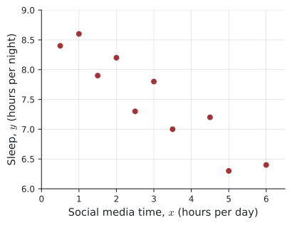
(a) Describe the correlation shown in the scatter diagram. [1]
(b) Find the value of the correlation coefficient \(r\). [2]
(c) Find the equation of the regression line of \(y\) on \(x\). [2]
(d) Interpret the gradient of this line in context. [1]
(e) Estimate the sleep of a student who spends \(4\) hours per day on social media. Comment on the reliability of your estimate. [3]
(f) Explain why the line should not be used for a student who spends \(10\) hours per day on social media. [1]
Another student sleeps \(7.0\) hours per night.
(g) Find the equation of a suitable regression line, justifying your choice, and use it to estimate this student’s social media time. [3]
A newspaper reports these results with the headline: “Cut your social media time and you will sleep longer.”
(h) Comment on the validity of this headline. [2]
Total 15 marks
(a)
strong negative linear correlation A1
Accept “fairly strong”. Both the direction and the strength are needed.
[1 mark]
(b)
\(r = -0.926\) \((-0.926036\ldots)\) (using Linear Regression (mx+b) on a GDC) A2
[2 marks]
(c)
\(y = -0.412x + 8.73\) \((-0.412147\ldots,\ 8.72583\ldots)\) A1 A1
[2 marks]
(d)
each extra hour per day on social media goes with about \(0.412\) hours (about \(25\) minutes) less sleep per night, on average A1
[1 mark]
(e)
\(y = -0.412147\ldots \times 4 + 8.72583\ldots = 7.08\) hours \((7.07724\ldots)\) A1
\(x = 4\) is inside the range of the data (\(0.5\) to \(6\) hours), so this is interpolation R1
and \(\lvert r \rvert = 0.926\) shows strong correlation, so the estimate is reliable R1
[3 marks]
(f)
\(10\) is far outside the range of the data (\(0.5\) to \(6\)), so this would be extrapolation R1
Accept a comment that the line gives \(4.60\) hours, but the linear pattern may not continue so far outside the data.
[1 mark]
(g)
\(y\) is given and \(x\) is to be estimated (neither variable is controlled), so use the regression line of \(x\) on \(y\) R1
\(x = -2.08y + 18.6\) \((-2.08067\ldots,\ 18.5758\ldots)\) (Linear Regression (mx+b) with the lists swapped) A1
\(x = -2.08067\ldots \times 7.0 + 18.5758\ldots = 4.01\) hours per day \((4.01114\ldots)\) A1
Accept \(4.04\) from the 3 s.f. coefficients. Do not award the last two marks for rearranging the line in (c), which gives \(4.19\).
[3 marks]
(h)
the headline is not valid: correlation does not imply causation R1
a third variable may affect both, for example students who go to bed late (or have more homework) may use social media more and also sleep less R1
[2 marks]
SL 5 Paper 2
On ten summer evenings, a biologist records the air temperature, \(T\) °C, and the mean number of chirps per minute, \(n\), made by crickets of one species. Neither variable is controlled.
| \(T\) (°C) | 14.2 | 16.0 | 17.5 | 18.1 | 19.6 |
|---|---|---|---|---|---|
| \(n\) | 74 | 79 | 96 | 90 | 112 |
| \(T\) (°C) | 21.0 | 22.4 | 23.8 | 25.5 | 27.0 |
|---|---|---|---|---|---|
| \(n\) | 105 | 126 | 128 | 152 | 147 |
(a) Find the value of the correlation coefficient \(r\), and interpret it in context. [2]
(b) Find the equation of the regression line of \(n\) on \(T\). [2]
(c) Interpret the gradient of this line in context. [1]
(d) Estimate the number of chirps per minute on an evening when the temperature is \(24\) °C. Comment on the reliability of your estimate. [2]
On another evening a hiker counts \(145\) chirps per minute.
(e) Estimate the temperature on that evening. Justify your choice of regression line. [3]
The biologist’s American colleague records the temperatures in degrees Fahrenheit, \(F\), where \(F = 1.8T + 32\).
(f) Write down the value of the correlation coefficient between \(F\) and \(n\), and find the equation of the regression line of \(n\) on \(F\). [4]
Total 14 marks
(a)
\(r = 0.974\) \((0.974115\ldots)\) (using Linear Regression (mx+b) on a GDC) A1
strong positive linear correlation: crickets tend to chirp faster on warmer evenings A1
[2 marks]
(b)
\(n = 6.30T - 18.3\) \((6.29938\ldots,\ -18.3004\ldots)\) A1 A1
[2 marks]
(c)
for each \(1\) °C rise in temperature, the crickets make about \(6.30\) more chirps per minute, on average A1
[1 mark]
(d)
\(n = 6.29938\ldots \times 24 - 18.3004\ldots = 133\) chirps per minute \((132.884\ldots)\) A1
reliable: \(24\) °C is inside the data (\(14.2\) to \(27.0\) °C) and \(r = 0.974\) shows strong correlation R1
[2 marks]
(e)
\(n\) is given and \(T\) is to be estimated, and neither variable is controlled, so use the regression line of \(T\) on \(n\) R1
\(T = 0.151n + 3.80\) \((0.150634\ldots,\ 3.80470\ldots)\) (Linear Regression (mx+b) with the lists swapped) A1
\(T = 0.150634\ldots \times 145 + 3.80470\ldots = 25.6\) °C \((25.6466\ldots)\) A1
Accept \(25.7\) from the 3 s.f. coefficients. Do not award the last two marks for rearranging the line in (b), which gives \(25.9\).
[3 marks]
(f)
\(r = 0.974\), the same as before, because \(F\) is a linear function of \(T\) with a positive multiplier A1
\(T = \dfrac{F - 32}{1.8}\), so \(n = 6.29938\ldots \times \dfrac{F - 32}{1.8} - 18.3004\ldots\) M1
\(n = 3.50F - 130\) \((3.49965\ldots,\ -130.289\ldots)\) A1 A1
Accept the line found by entering the values of \(F\) on a GDC.
[4 marks]
HL questions
This unit has no AHL content, so the HL questions test the same syllabus content as SL, but they are longer and need more careful reasoning about least squares and the mean point.
HL 1 Paper 1
A set of nine pairs of data \((x, y)\) has \(\bar{x} = 10\). The regression line of \(y\) on \(x\) is \(y = 1.5x + 4\), and the regression line of \(x\) on \(y\) is \(x = 0.6y - 1.4\).
(a) Find \(\bar{y}\). [1]
A tenth pair, \((20, 34)\), is added to the data.
(b) Find the mean point of the ten pairs. [2]
The regression line of \(y\) on \(x\) is the line that makes the sum of the squares of the vertical distances from the points to the line as small as possible.
(c) Explain why the regression line of \(y\) on \(x\) for the ten pairs is still \(y = 1.5x + 4\). [3]
(d) Show that the regression line of \(x\) on \(y\) for the ten pairs is not \(x = 0.6y - 1.4\). [2]
Total 8 marks
(a)
\(\bar{y} = 1.5 \times 10 + 4 = 19\) A1
[1 mark]
(b)
\(\sum x = 9 \times 10 + 20 = 110\) and \(\sum y = 9 \times 19 + 34 = 205\) M1
mean point \((11, 20.5)\) A1
[2 marks]
(c)
\(1.5 \times 20 + 4 = 34\), so the new point lies on the line: its vertical distance from the line is \(0\) R1
so for the line \(y = 1.5x + 4\) the sum of squares is the same as for the nine pairs R1
for any other line the new sum is at least its sum for the nine pairs, which is at least the sum for \(y = 1.5x + 4\); so \(y = 1.5x + 4\) still gives the smallest sum R1
Showing only that \((11, 20.5)\) lies on \(y = 1.5x + 4\) is not enough: many lines pass through the mean point.
[3 marks]
(d)
the regression line of \(x\) on \(y\) for the ten pairs must pass through the new mean point \((11, 20.5)\) R1
\(0.6 \times 20.5 - 1.4 = 10.9 \neq 11\), so \(x = 0.6y - 1.4\) does not pass through it, and the line has changed A1
[2 marks]
See 17.2.
HL 2 Paper 1
Five pairs of data are shown.
| \(x\) | 1 | 2 | 3 | 4 | 5 |
|---|---|---|---|---|---|
| \(y\) | 3 | 4 | 8 | 9 | 11 |
The least-squares regression line of \(y\) on \(x\) passes through the mean point \((\bar{x}, \bar{y})\). Consider a line through \((\bar{x}, \bar{y})\) with gradient \(m\). Let \(S(m)\) be the sum of the squares of the vertical distances from the five points to this line.
(a) Show that \(S(m) = 10m^{2} - 42m + 46\). [4]
(b) Hence find the equation of the regression line of \(y\) on \(x\). [3]
(c) Find the least possible value of \(S(m)\). [1]
Total 8 marks
(a)
\(\bar{x} = \dfrac{15}{5} = 3\) and \(\bar{y} = \dfrac{35}{5} = 7\) A1
the line is \(y = 7 + m(x - 3)\); the vertical distance of \((x, y)\) from it is \(\lvert (y - 7) - m(x - 3) \rvert\) M1
\(x - 3\): \(-2, -1, 0, 1, 2\) and \(y - 7\): \(-4, -3, 1, 2, 4\) A1
\(S(m) = (2m - 4)^{2} + (m - 3)^{2} + 1^{2} + (2 - m)^{2} + (4 - 2m)^{2}\) M1
\(= (4m^{2} - 16m + 16) + (m^{2} - 6m + 9) + 1\)
\(\quad + (m^{2} - 4m + 4) + (4m^{2} - 16m + 16)\)
\(= 10m^{2} - 42m + 46\) AG
[4 marks]
(b)
\(S(m)\) is a quadratic with a positive coefficient of \(m^{2}\), so its minimum is at the vertex: \(m = \dfrac{42}{2 \times 10}\) M1
\(m = 2.1\) A1
\(y - 7 = 2.1(x - 3)\), so \(y = 2.1x + 0.7\) A1
[3 marks]
(c)
\(S(2.1) = 10(2.1)^{2} - 42(2.1) + 46 = 1.9\) A1
[1 mark]
See 17.2.
HL 3 Paper 2
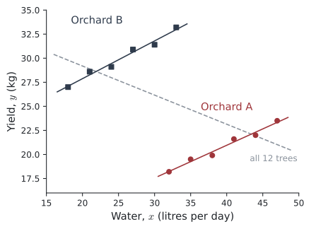
A fruit farmer has two orchards. Orchard A is in a hot, dry valley, and orchard B is on a cooler hillside. For six trees in each orchard she chooses the amount of water given to the tree, \(x\) litres per day, and records the yield of fruit, \(y\) kg.
Orchard A:
| \(x\) | 32 | 35 | 38 | 41 | 44 | 47 |
|---|---|---|---|---|---|---|
| \(y\) | 18.2 | 19.5 | 19.9 | 21.6 | 22.0 | 23.5 |
Orchard B:
| \(x\) | 18 | 21 | 24 | 27 | 30 | 33 |
|---|---|---|---|---|---|---|
| \(y\) | 27.0 | 28.6 | 29.1 | 30.9 | 31.4 | 33.2 |
(a) Find the correlation coefficient \(r\) for orchard A and for orchard B. [2]
(b) Find the correlation coefficient for all twelve trees together. [1]
(c) The farmer looks only at the combined data for all twelve trees. She concludes that giving a tree more water tends to reduce its yield. Explain why this conclusion is not valid. [2]
(d) Find the equation of the regression line of \(y\) on \(x\) for orchard B, and use it to estimate the yield of a tree in orchard B that is given \(25\) litres of water per day. [3]
Total 8 marks
(a)
orchard A: \(r = 0.989\) \((0.988626\ldots)\) (using Linear Regression (mx+b) on a GDC) A1
orchard B: \(r = 0.989\) \((0.989364\ldots)\) A1
[2 marks]
(b)
\(r = -0.525\) \((-0.524726\ldots)\) A1
[1 mark]
(c)
within each orchard there is a very strong positive correlation: more water goes with a larger yield R1
the negative value for the combined data comes from a third variable (the orchard and its climate): the trees in the hot valley are given more water but give less fruit R1
[2 marks]
(d)
\(y = 0.392x + 20.0\) \((0.392381\ldots,\ 20.0276\ldots)\) A1 A1
\(y = 0.392381\ldots \times 25 + 20.0276\ldots = 29.8\) kg \((29.8371\ldots)\) A1
[3 marks]
HL 4 Paper 2
The table shows the mathematics mark, \(x\), and the physics mark, \(y\), of nine students A to I in the same term. Neither variable was controlled.
| Student | A | B | C | D | E |
|---|---|---|---|---|---|
| \(x\) | 45 | 52 | 58 | 61 | 66 |
| \(y\) | 41 | 50 | 55 | 26 | 63 |
| Student | F | G | H | I |
|---|---|---|---|---|
| \(x\) | 70 | 74 | 81 | 88 |
| \(y\) | 64 | 71 | 75 | 84 |
(a) Find the value of the correlation coefficient \(r\) for these nine students. [2]
(b) Find the equation of the regression line of \(y\) on \(x\). Hence show that student D’s physics mark is more than \(25\) marks below the value predicted by this line. [3]
The teacher finds that D’s physics mark was recorded incorrectly. The correct mark is \(59\).
(c) For the corrected data, find the value of \(r\). Comment on the effect that the error had on \(r\). [2]
(d) For the corrected data, find the equation of the regression line of \(y\) on \(x\) and the equation of the regression line of \(x\) on \(y\). [4]
(e) Estimate the physics mark of a student whose mathematics mark is \(77\). [1]
(f) Estimate the mathematics mark of a student whose physics mark is \(50\). Justify your choice of line. [2]
(g) Write down the coordinates of the point where the two lines in part (d) intersect. Give a reason for your answer. [2]
Total 16 marks
(a)
\(r = 0.814\) \((0.813673\ldots)\) (using Linear Regression (mx+b) on a GDC) A2
[2 marks]
(b)
\(y = 1.06x - 11.4\) \((1.06095\ldots,\ -11.3628\ldots)\) A1
at \(x = 61\): \(\;y = 1.06095\ldots \times 61 - 11.3628\ldots = 53.355\ldots\) M1
\(53.355\ldots - 26 = 27.4 > 25\) A1 AG
[3 marks]
(c)
\(r = 0.995\) \((0.994859\ldots)\) A1
one wrong value made the correlation look much weaker (\(0.814\) instead of \(0.995\)) R1
[2 marks]
(d)
\(y = 0.950x - 0.335\) \((0.949611\ldots,\ -0.335411\ldots)\) A1 A1
\(x = 1.04y + 1.03\) \((1.04226\ldots,\ 1.02753\ldots)\) (with the lists swapped) A1 A1
[4 marks]
(e)
\(y = 0.949611\ldots \times 77 - 0.335411\ldots = 72.8\) \((72.7847\ldots)\) A1
[1 mark]
(f)
\(y\) is given and \(x\) is to be estimated (neither variable is controlled), so use the line of \(x\) on \(y\) R1
\(x = 1.04226\ldots \times 50 + 1.02753\ldots = 53.1\) \((53.1407\ldots)\) A1
Accept \(53.0\) from the 3 s.f. coefficients.
[2 marks]
(g)
both regression lines pass through the mean point \((\bar{x}, \bar{y})\) R1
\(\left(\dfrac{595}{9}, \dfrac{562}{9}\right) = (66.1, 62.4)\) \((66.111\ldots,\ 62.444\ldots)\) A1
Accept the point found by solving the two equations, for example using the intersection of the two graphs on a GDC.
[2 marks]
HL 5 Paper 1
A power company records, on \(12\) summer days, the maximum temperature, \(x\) °C, and the electricity used in a town, \(y\) megawatt-hours (MWh). The temperatures were between \(22\) °C and \(34\) °C, and neither variable was controlled. For these data, \(\displaystyle\sum x = 336\).
The regression line of \(y\) on \(x\) is \(y = 3.6x + 49.2\). The regression line of \(x\) on \(y\) has gradient \(0.2\).
(a) Find \(\bar{x}\) and \(\bar{y}\). [3]
(b) Interpret the value \(3.6\) in context. [1]
(c) Find the equation of the regression line of \(x\) on \(y\). [2]
(d) On one day the town used \(160\) MWh of electricity. Estimate the maximum temperature on that day. Justify your choice of line. [2]
(e) Use the regression line of \(y\) on \(x\) to estimate the electricity used on a day with a maximum temperature of \(41\) °C. Comment on your answer. [2]
The company’s engineers record temperatures in degrees Fahrenheit, \(F\), where \(F = 1.8x + 32\).
(f) Show that the regression line of \(y\) on \(F\) is \(y = 2F - 14.8\). [3]
(g) Find the equation of the regression line of \(F\) on \(y\). [2]
(h) Explain why the correlation coefficient between \(F\) and \(y\) is equal to the correlation coefficient between \(x\) and \(y\). [1]
Total 16 marks
(a)
\(\bar{x} = \dfrac{336}{12} = 28\) A1
the line passes through \((\bar{x}, \bar{y})\): \(\;\bar{y} = 3.6 \times 28 + 49.2\) M1
\(\bar{y} = 150\) A1
[3 marks]
(b)
for each \(1\) °C rise in the maximum temperature, the town uses about \(3.6\) MWh more electricity, on average A1
[1 mark]
(c)
\(x = 0.2y + d\) passes through \((28, 150)\): \(\;28 = 0.2 \times 150 + d\) M1
\(d = -2\), so \(x = 0.2y - 2\) A1
[2 marks]
(d)
\(y\) is given and \(x\) is to be estimated, so use the line of \(x\) on \(y\) R1
\(x = 0.2 \times 160 - 2 = 30\) °C A1
[2 marks]
(e)
\(y = 3.6 \times 41 + 49.2 = 196.8\) MWh A1
not reliable: \(41\) °C is outside the data (\(22\) to \(34\) °C), so this is extrapolation R1
[2 marks]
(f)
\(x = \dfrac{F - 32}{1.8}\) M1
\(y = 3.6 \times \dfrac{F - 32}{1.8} + 49.2 = 2(F - 32) + 49.2\) A1
\(y = 2F - 64 + 49.2 = 2F - 14.8\) A1 AG
A linear change of units only stretches and moves the scatter diagram, so the regression line is changed in the same way.
[3 marks]
(g)
\(F = 1.8x + 32 = 1.8(0.2y - 2) + 32\) M1
\(F = 0.36y + 28.4\) A1
[2 marks]
(h)
\(F = 1.8x + 32\) is a linear change of scale with a positive multiplier (\(1.8 > 0\)), so \(r\) does not change R1
[1 mark]